Tuning and Costs Analysis for a Trajectory Planning Algorithm for

Autonomous Vehicles

Abdallah Said

1,2

, Reine Talj

, Clovis Francis

and Hassan Shraim

Universit

e de Technologie de Compi

egne, CNRS, Heudiasyc (Heuristics and Diagnosis of Complex Systems), CS 60 319,

60 203 Compi

egne Cedex, France

Universit

e Lebanonaise, Facult

e de G

enie, Centre de Recherche Scientiﬁque en Ing

enierie (CRSI), Lebanon

Keywords:

Autonomous Vehicle, Trajectory Planning, Cost Analysis.

Abstract:

Trajectory planning is an essential issue for autonomous vehicles navigation. It represents a decision-making

level that considers several constraints to be respected to navigate safely and comfortably in a dynamic en-

vironment. This paper presents a reactive trajectory planning, which consists to generates several candidate

trajectories. Then, selecting the best trajectory among candidates is based on different criteria, each described

by a cost function. Indeed, the algorithm aims to minimize a global cost function, a combination of several

costs, to determine the best trajectory. The main objective of this work is to study the algorithm’s sensitiv-

ity against parameter tuning and to ﬁnd a generic range of weighting coefﬁcients for the cost function of the

planning algorithm to make the algorithm as reliable as possible against various driving conditions.

1 INTRODUCTION

An autonomous vehicle needs a local trajectory based

on real-time vehicle status and dynamic environment

perception data (e.g., nearby cars, road conditions) to

guarantee safe maneuvers while following the global

trajectory. Local trajectory planning is deﬁned as the

planning of a vehicle’s transition from one possible

state to the next one while satisfying the vehicle’s

kinematic restrictions based on the vehicle dynam-

ics and constrained by the passenger’s comfort, lane

boundaries, and trafﬁc rules while avoiding static and

dynamic obstacles. Different trajectory planning ap-

proaches have been developed for the navigation of

autonomous vehicles (Dixit et al., 2018), (Katrakazas

et al., 2015). They differ in how they deal with the en-

vironment and the vehicle dynamics limitations. Ac-

cording to the literature, there are four well-known

approaches to trajectory planning methods: grids gen-

eralization (Pivtoraiko and Kelly, 2005), sampling-

based planning (Karaman and Frazzoli, 2011), nu-

merical optimization methods (Lim et al., 2018) and

curve interpolation methods (Alia et al., 2015). The

last approach is adopted, and it aims to generate tra-

jectories on a given horizon with a speciﬁed geomet-

ric shape that responds to one or more constraints

such as vehicle dynamics and kinematics, comfort,

road shape, and curvature continuity. Each candidate

trajectory is assessed using a cost function that takes

into account several factors such as traveled distance

and execution time costs, acceleration, collision ver-

iﬁcation, and other performance criteria. Then, the

cost function is minimized to ﬁnd the best trajectory

among several candidate trajectories generated by the

planning algorithm. Each one of these costs is mul-

tiplied by a weighting coefﬁcient to rank its signiﬁ-

cance. The major weakness of this approach is that,

for some trajectory shapes, the result of the planning

algorithm is highly dependent on the tuning of the

cost weights . Moreover, function of the shape of

geometric curves, which represent candidate trajecto-

ries, the algorithm is more or less dependent on tun-

ing weights. It is important to evaluate the sensitiv-

ity of the planning algorithm to the tuning parame-

ters in order to evaluate its ability to deal with the

different driving situations without the need to adapt

the parameters. In (Zhang et al., 2018), the planner’s

ﬂexibility is deﬁned by how many different types of

scenarios it can manage by just altering parameters

rather than modifying the fundamental issue formu-

lation or problem structures. In (Mouhagir et al.,

2017), trajectory planning based on clothoid tentacles

was adopted. Different combinations for cost func-

tion weights were proposed and the results show that

the proposed method was very sensitive to parameter

variation and some combinations were not suitable for

Said, A., Talj, R., Francis, C. and Shraim, H.

Tuning and Costs Analysis for a Trajectory Planning Algorithm for Autonomous Vehicles.

DOI: 10.5220/0011067700003191

In Proceedings of the 8th International Conference on Vehicle Technology and Intelligent Transport Systems (VEHITS 2022), pages 88-95

ISBN: 978-989-758-573-9; ISSN: 2184-495X

real-time application. A study is presented in (Arnay

et al., 2016) on the impact of the weights of a cost

function with ﬁve criteria on the ﬁnal behavior of the

vehicle. This planner deals with only pedestrians as

obstacles and low velocities. Several conﬁgurations

were chosen and ranked based on two behaviors.

In order to choose the best combination of

weights, the role of each cost must be investigated and

its inﬂuence in choosing the best candidate trajectory

must be understood. In this paper, impact analysis

and tuning of weighting coefﬁcients are done on the

planning algorithm presented in (Said et al., 2021).

This paper is organized as follows: in Section 2, we

present the trajectory planning algorithm. The global

cost function and its components are detailed in Sec-

tion 2.2. Section 3 presents the proposed method and

reports the simulation results with some analysis on

the cost weights, while the ﬁnal Section 4 concludes

the paper.

2 TRAJECTORY PLANNING

2.1 Presentation of the Trajectory

Planning Method

The trajectory planning algorithm must provide the

best trajectory from a set of candidate trajectories

that helps the vehicle to track a reference trajectory

while avoiding static and mobile obstacles and ensur-

ing safety and passenger comfort. Fig.1 shows the lo-

cal trajectory planning module. Starting from match-

Generation of

candidate paths

Obstacle detection

and path

classification

Selection of the

optimal path

Cost calculation

Figure 1: Local trajectory planning module.

ing the vehicle on the reference trajectory, a set of

candidate trajectories are generated. they cover either

the host lane or the entire width of the road depend-

ing on their navigability. Each of them consists of

two phases: The transient phase, which is modeled

by a 4

order polynomial curve to provide a smooth

change ensuring continuity of the curvature, starts at

the actual position of the vehicle up to a deﬁned lateral

offset from the reference trajectory. Then, the candi-

date trajectory continues with a permanent phase par-

allel to the reference trajectory where the lateral offset

becomes constant (see Fig. 2). Secondly, an obstacle

detection procedure is carried out. A classiﬁcation

area is formed along the candidate trajectory by the

footprint of the vehicle. The collision distance d

obs

which is the free distance traveled on the trajectory to

reach the ﬁrst obstacle, is then detected. Based on the

collision distance and security distance, we classify

the candidate trajectories into three classes: non, par-

tially, or fully navigable trajectory. Note that the secu-

rity distance is the distance the vehicle must maintain

between it and the encountered obstacle. It depends

on the obstacle state (static or dynamic). It is calcu-

lated based on the safe stop distance, the needed dis-

tance to stop the vehicle from its actual speed, with a

deﬁned comfortable deceleration. If there are no nav-

igable trajectories, the algorithm selects the one with

the longest distance to the obstacle to stop the vehicle

with high deceleration (safe stop scenario). Thirdly,

the navigable trajectories are evaluated according to

various criteria, including smoothness, safety, consis-

tency with the previously selected trajectory of the ve-

hicle, and tracking of the reference center lane. All

these costs are detailed in Section 2.2. Once these cri-

teria are costed and merged into a weighted global

cost function, the chosen trajectory is the best one

with the lowest cost. Finally, a set of points, deﬁned

by the curvilinear abscissa, x and y coordinates, ve-

locity, and curvature, depicts the best trajectory. For

more details on the planning algorithm and its imple-

mentation, please refer to (Said et al., 2021).

2.2 Cost Function Deﬁnition

The cost function is a weighted combination of costs

that should be minimized in order to ﬁnd the best tra-

jectory among the many candidate trajectories gener-

ated by the planning algorithm. These costs are:

1. Smoothness Cost C

[i]:

This cost seeks to prefer lower-curvature trajecto-

ries. On the other hand, soft smoothness causes

increased lateral acceleration, which affects pas-

senger comfort. As a result, the integration of the

curvature squared along a trajectory is chosen as

a smoothness requirement for this trajectory in or-

der to reduce its slackness:

[i] =

(1)

Figure 2: Trajectory planning: simulation environment.

Tuning and Costs Analysis for a Trajectory Planning Algorithm for Autonomous Vehicles

where ρ

and ds

are the curvature and the curvi-

linear abscissa of a point M along the candidate

trajectory i, respectively.

2. Cost of Tracking the Reference Trajectory

[i]:

In order to position the ego vehicle in the center

of the intended lane, the vehicle must follow the

global reference trajectory. The cost of follow-

ing the reference trajectory is related to the offset

since the candidate trajectories are created around

this lane center with a given lateral offset (Fig. 2).

The reference cost in multi-lane structured envi-

ronment is determined by the vehicle’s position

in relation to the lanes. So, the reference cost is

given by:

[i] = (q

−q

re f c

)

, (2)

where q

is the lateral shift of the permanent

phase of the candidate trajectory i to the host lane,

re f c

is the lateral offset of the center of the ref-

erence lane. By default, the reference lane is the

one in which the vehicle is located: it is either the

host lane (q

re f c

= 0) or adjacent lane (q

re f c

= q

However, in case of returning to the host lane in

an obstacle overtaking scenario, the host lane be-

comes the reference if the vehicle passes the ob-

stacle (dotted lane in Fig.3) and the host lane is

navigable. Fig.3 shows the different cases for the

deﬁnition of the reference lane.

Figure 3: Reference cost cases.

3. Consistency Cost C

[i]:

A quick shift in the selected trajectory between

two iterations needs a considerable control effort

and can affect the vehicle’s stability. As a result, a

measure of similarity between the prior trajectory

and the current candidate trajectory is required to

avoid generating a trajectory that is drastically dif-

ferent from that of the previous step. Our tech-

nique reduces it to the difference between the cur-

rent trajectory index i and the chosen one from a

prior planning iteration.

[i] = |i −i

t−1

des

| (3)

4. Safety Cost C

[i]:

We deﬁne two safety costs: a longitudinal cost C

and a lateral cost C

. The ﬁrst one assesses the

trajectory’s navigability and the distance to the

ﬁrst obstacle. This cost increases when the ﬁrst

detected obstacle is longitudinally close and de-

creases when the obstacle is far (Fig. 4-left). The

second cost considers the navigability of nearby

trajectories and attempts to position the vehicle

laterally in the middle of the navigable zone. The

collision distance d

obs

(distance to the ﬁrst obsta-

cle) is transformed into a safety cost as follows:

[i] =

(

0 obstacle-free trajectory

2 −

1+e

−c

obs

otherwise

(4)

g[k] =

√

2πσ

exp



−

(k ∆q)

2σ



(5)

[i] = (

∑

j∈Γ

[ j] g[i − j]) /n

(6)

where c

is a cost setting parameter, ∆q is the de-

sired lateral sampling resolution, σ is the standard

deviation of the discrete Gaussian convolution for

the risk of collision and is calculated by consider-

ing that g[

∆q

] = 0.5, where L

is the vehicle width

(Fig. 4-right). Γ

is the set of indexes of generated

trajectories without i, n

is their number.

Figure 4: Safety cost.

Total Cost Function C

[i]:

We use the normalization technique to make the dif-

ferent cost criteria dimensionless because they are as-

sessed in different units. As a result, we use the fol-

lowing formula:

[i] =

[i] −min(C

)

max(C

) −min(C

)

(7)

Then, the total cost function C

[i] of a given tra-

jectory is deﬁned as the weighted sum of the normal-

ized cost functions deﬁned above:

[i] =W

[i] +W

[i]

[i] +W

[i]

(8)

with W

, W

and W

the weighting coef-

ﬁcients of smoothness, consistency, reference track-

ing, longitudinal safety and lateral safety costs respec-

tively.

VEHITS 2022 - 8th International Conference on Vehicle Technology and Intelligent Transport Systems

3 IMPACT ANALYSIS AND

TUNING OF WEIGHTING

COEFFICIENTS

3.1 Proposed Method

Our goal is to understand better each cost inﬂuence

on choosing the best trajectory and to ﬁnd a generic

weighting coefﬁcients range for the cost function of

the planning algorithm. First, we propose scenarios

with or without static or dynamic obstacles. Second,

we generate n random combinations of weighting co-

efﬁcients, each weight is bounded between two values

(0 ≤ l

≤W

≤u

≤1). The random method was used

due to the high number of combinations in a classic

grid search method with ﬁve weights. Then, we run

the planning algorithm n times. The n vehicle’s tra-

jectories obtained are classiﬁed into two categories:

• T

complete vehicle’s trajectory set: the algorithm

manages to reach the end of the proposed scenario

without stopping or colliding with any obstacle.

• T

incomplete vehicle’s trajectory set: the algo-

rithm fails to reach the end of the proposed sce-

nario due to hitting an obstacle or lane’s borders.

The correlation between the obtained results and the

corresponding combinations is then analyzed accord-

ing to various factors such as the distance traveled, the

longitudinal and the lateral acceleration, the reference

tracking, the safety distance, and the overall behavior

(conservative or aggressive). Based on this analysis,

the wide range chosen ﬁrst is contracted. this proce-

dure is repeated until we obtain the desired generic

range.

3.2 Case Study

To study the proposed method, we apply the plan-

ning algorithm on a portion of a realistic trajectory

track taken from SCANeR

T M

studio simulator, with

different scenarios, for 50 random combinations. This

trajectory and the corresponding limit speed and cur-

vature are shown in Fig. 5. Initial speed may vary

depending on the scenario. The trajectory planning

module is implemented in an autonomous driving sys-

tem composed of main modules for navigation: lo-

calization, perception, trajectory planning, control,

and vehicle model. The two last modules are run-

ning at 50 Hz while the others are running at 10 Hz.

The Renault-Zoe robotic vehicle model validated on

SCANeR

T M

studio is used.

The presented scenarios are simulated using the

combinations of weighting coefﬁcients presented in

Fig. 6. We start with simple scenarios and large

Figure 5: Trajectory, longitudinal speed and curvature

(same legend as Fig. 2).

ranges for weighting coefﬁcients. The smoothness,

reference, and consistency coefﬁcients ranges are

chosen to be between 5% and 40% as they are used for

performance purposes,while the coefﬁcients ranges of

safety costs are greater: The longitudinal safety one

is between 5% and 65%. The lateral safety one is be-

tween 5% and 50%. These ranges are chosen based

on evident knowledge about the algorithm and pre-

liminary simulations. Safety is prior to performance

while deciding the trajectory for autonomous naviga-

tion. Outside of these ranges, the planning algorithm

does not give reasonable trajectories that can be ex-

ecuted. It will either give an extremely smooth with

high smoothness weight or aggressive trajectory with

high reference weight that will try to follow the lane’s

center.

Figure 6: Box plot of 50 combinations of weighting coefﬁ-

cients.

In the following, for each scenario, we illustrate

the generated trajectories for all combinations and the

ﬁnal reached points for the same time horizon in order

to analyze the results.

3.2.1 Scenario 1: Static Obstacle Overtaking

The scenario presented in Fig. 7 consists of an over-

taking of two static obstacles, each one on a lane sep-

Tuning and Costs Analysis for a Trajectory Planning Algorithm for Autonomous Vehicles

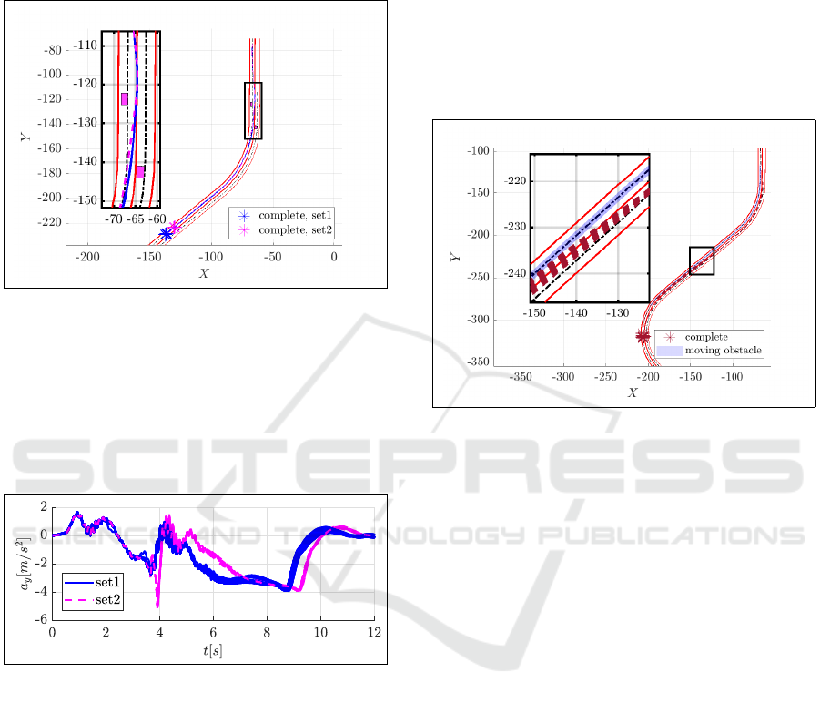
arated by a distance of 15m. This distance is con-

sidered small, taking into account the lane’s desired

speed (65km/h), and for this, the algorithm pushes the

vehicle to brake when it slaloms between obstacles.

Figure 7: Scenario 1: trajectories in presence of 2 static

obstacles (same legend as Fig. 2).

In some combinations, where the sum of smooth-

ness and consistency weights is signiﬁcant (Set 2:

> 12% or W

> 13% ), the vehicle crosses the

trajectory with a high lateral acceleration value (>

4m/s

) as shown in set 2 in Fig. 8, where set 1 repre-

sents trajectories with the remaining combinations.

Figure 8: Scenario 1: lateral acceleration.

The smoothness cost leads the vehicle to move

straight towards the obstacle, especially if the longitu-

dinal safety weighting coefﬁcient is too small. In con-

trast, the consistency cost delays the lane change until

the last possible moment before reaching the safe stop

distance, and this results in strong lateral acceleration.

Then the algorithm proceeds to additional braking to

ensure lateral stability. We note here that the devel-

oped algorithm is able to execute the trajectory safely,

even with small safety weighting coefﬁcients. As we

can see in Fig. 7, all trajectories can reach the end

of the scenario, and with almost a 10m difference be-

tween their ends due to additional braking on some

trajectories (set 2). However, we can note that the

trajectories with high lateral safety (W

> 40%) and

reference (W

> 20%) weighting coefﬁcients execute

the longest distance and hence offers the highest lon-

gitudinal speed.

3.2.2 Scenario 2: Mobile Obstacle Overtaking

The second scenario is a simple overtaking of a mo-

bile obstacle at 40km/h where the vehicle speed dur-

ing overtaking reaches 50 to 60km/h. As we can see

in Fig. 9, all trajectories can reach the end of the sce-

nario.

Figure 9: Scenario 2: trajectories in a mobile obstacle over-

taking (same legend as Fig. 2).

The difference between trajectories can be seen in

Fig. 10 when overtaking and returning to the host

lane. The security inter-distance is respected in all

combinations but leads to more or less conservative

behavior depending on the reference weighting coef-

ﬁcient. For all combinations, the vehicle starts over-

taking before 35m, which is the security distance cor-

responding to its velocity. However, the overtaking

starts earlier with a high lateral safety weight. How-

ever, when returning to the lane, the inter-distance of

the ﬁrst trajectory that reaches the host lane’s center

is equal to 22m, which is equal to 2 seconds of ob-

stacle’s speed. Set 4 in Fig.10 represents trajectories

with smoothness weight W

higher than > 30%.

In this set, the three trajectories with a late return

to the lane have in addition a low reference weight

< 7%, while the rest of the trajectories try hard to

follow the center of the track.

Furthermore, the reference cost acts on the ve-

hicle stability: a high reference weight with low

smoothness or consistency weight (set5: W

> 15%

and (W

< 6% or W

< 6%) ) leads to a higher lat-

eral acceleration compared to other combinations (see

Fig.11) and may result in a passenger’s discomfort,

due to late change lane and rapid return to the host

lane.

Note that set 3 represents trajectories with the re-

VEHITS 2022 - 8th International Conference on Vehicle Technology and Intelligent Transport Systems

maining combinations.

Figure 10: Scenario 2: Frenet frame.

Figure 11: Scenario 2: lateral acceleration.

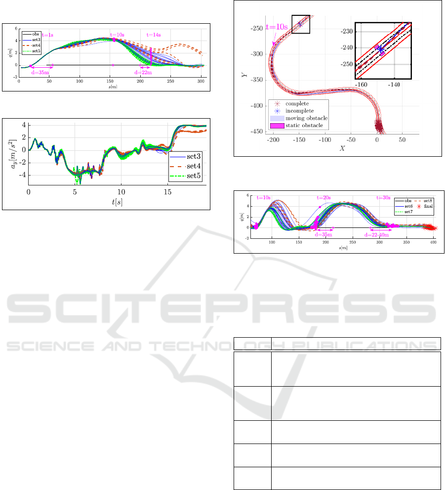
3.2.3 Scenario 3.1: Multi-maneuver Scenario

This scenario combines several maneuvers: reference

tracking, tight passage, static obstacle overtaking with

a mobile obstacle on the adjacent lane in the opposite

direction (t = 10s), and mobile obstacle overtaking

(t = 20s).

As we can see in Fig.12, 92% of the generated

trajectories can complete the scenario.

The incomplete trajectories fail at the tight pas-

sage: the classiﬁcation area around the trajectory,

which is a little larger than the vehicle’s imprint, de-

tects hitting one of the obstacles. The four failed com-

binations have low lateral safety weights ( W

< 10%)

value and high reference weight (W

> 30%).

This result is expected as the reference cost forces

the vehicle to track the reference lane while the lateral

safety cost tries to pass it in the middle of the naviga-

ble zone.

Fig.13 represents the generated trajectories in the

Frenet frame. We can see a signiﬁcant difference

between the trajectories. After t = 10s, we notice

that a high reference and lateral safety weights (set

7: W

> 18% and W

> 30%) lead to an early re-

turn to the host lane, while those with low reference

weight and high smoothness weights (set 8: W

< 8%

and W

> 25%) were late to return and overtake. In

addition, the last one to return was the one with a

high value of smoothness weight (W

= 39%) and

caused over-steering when trying to follow the ref-

erence (s = 170m). At the overtaking of the mobile

obstacle (t = 20s), the high lateral safety weight leads

to earlier overtaking and then to an earlier return to

the lane. The longest trajectories were those with the

Figure 12: Scenario 3.1: trajectories (same legend as Fig.

2).

Figure 13: Scenario 3.1: Frenet frame.

high lateral safety weight (W

= 45% of the longest

one). Note that set 6 represents trajectories with the

remaining combinations.

Table 1: Cost analysis results.

cost result

high value of smoothness weight leads

to a late lane change, high a

and

over/under steer

high value of reference weight leads to

an early lane change, high a

, prioritize

reference tracking over safety

high consistency weight leads to high a

(> 0.4g)

high lateral safety weight leads to

longest path, early lane change;

longitudinal safety weight has a similar

effect to lateral safety ;

From these results, we can deduce that the

smoothness, reference, and consistency weighting co-

efﬁcients should be limited to relatively small values.

Indeed, a high reference weight coefﬁcient can be ag-

gressive in a dual lane change scenario. Furthermore,

high smoothness and consistency weights may cause

a delay in response to the change in curvature. Con-

sequently, bounded combinations are applied in the

following simulation scenario.

Tuning and Costs Analysis for a Trajectory Planning Algorithm for Autonomous Vehicles

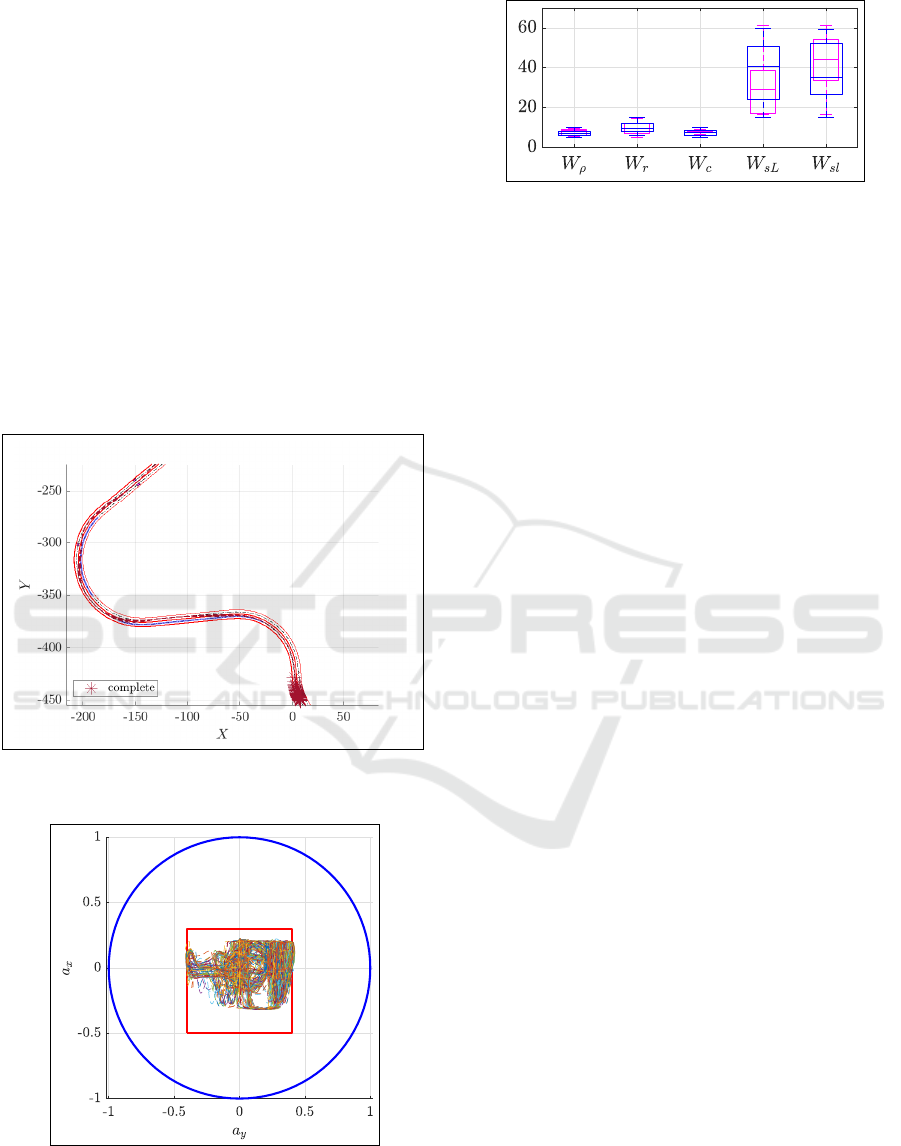
3.2.4 Scenario 3.2: Multi-maneuver Scenario

with Limited Combinations

After many tests and simulations, we decided to limit

the ranges of weighting coefﬁcients around the most

favorable values. The new range proposed for combi-

nations of weighting coefﬁcients is between 5% and

10% for smoothness and consistency cost’s weights,

between 5% and 15% for reference cost’s weight, and

between 15% and 65% for longitudinal and lateral

safety cost’s weights.

These new ranges are applied to the same scenario

of 3.2.3. As we can see in Fig. 14, all trajectories can

reach the end of the scenario, and the difference at

the arrival point is less than 5m for different combina-

tions of trajectories. In addition, it shows that all tra-

jectories can pass smoothly and follow the reference

without any accident.

Figure 14: Scenario 3.2: trajectories (same legend as Fig.

2).

Figure 15: g-G diagram for 50 combinations in a 0.4g red

box.

Using a normalized friction circle and the g-g dia-

gram, we show that the planning algorithm can main-

normal A

:44/50;

high A

:6/50

Figure 16: Box plot of combinations of weighting coefﬁ-

cients.

tain the vehicle for all combinations in the comfort

region (red rectangle in Fig.15). A classiﬁcation of

combinations based on maximal lateral acceleration

reached with a threshold of 0.38g is done. The results

are illustrated using the box plot shown in Fig.16: A

high lateral acceleration is reached with a low lateral

safety weight and a high reference weight. This be-

havior is expected due to the late lane change. Note

that even the combinations presenting high lateral ac-

celeration values still have an acceleration less than

0.4g as shown in Fig.15.

Note that these combinations are simulated for all

the previous scenarios and succeed in reaching their

ends.

3.2.5 Scenario 3.3: Longitudinal and Lateral

Safety Costs

To better understand the impact of the two compo-

nents of the safety cost of the algorithm behavior,

we simulate the third scenario with a ﬁxed value for

smoothness, reference, and consistency weights as

8%, 14% and 8% respectively, while the range of the

two safety costs is between 15% and 65%.

All combinations succeed in ﬁnishing the scenario

smoothly with a lateral acceleration inside the com-

fort zone.

3.3 Discussion about Costs Inﬂuence

Correlation

The results presented above give us a better under-

standing of the different costs that inﬂuence choos-

ing the best trajectory. These simulations helped us

to improve the planning algorithm. A good combina-

tion weight coefﬁcients leads the vehicle to track the

reference lane and to overtake smoothly and safely

in the presence of obstacles, when overtaking is pos-

sible, without an abrupt lane change. Moreover, the

planning algorithm respects the safety distances with

all static and mobile obstacles and stops the vehicle

if needed when no navigable trajectory is detected.

The smoothness cost, as deﬁned, tries to move the ve-

hicle straight forward as much as possible. Unfor-

VEHITS 2022 - 8th International Conference on Vehicle Technology and Intelligent Transport Systems

tunately, it delays the lane return with low reference

cost or high consistency cost. The consistency cost

acts as a damper of the vehicle’s motion by delaying

the variation of the vehicle’s orientation. Concern-

ing the reference cost, it plays an essential role, as

presented before in all the scenarios. When encoun-

tering an obstacle, a high reference weight causes a

high lateral acceleration, especially for the combina-

tion where the consistency or smoothness weight is

low or the lateral safety weight is low. The safety

cost guides the vehicle very well in the navigable zone

and respects the inter-distances. In some cases, the

costs identiﬁed above may correlate with each other.

For example, in the case of lane following, the lateral

safety cost correlates with the reference tracking cost

by maximizing the lateral safety cost of candidate tra-

jectories near the lane borders and thus minimizing

those towards the lane’s center. On the other hand,

they behave differently when the lateral safety cost

tries to position the vehicle in the middle of the navi-

gable zone, away from the reference lane. The higher

is the reference cost; the earlier is the host lane track-

ing. Finally, choosing the different weights of the cost

function components must obey to a compromise be-

tween the other considered criteria. It is crucial to

prioritize safety on performance. The present analy-

sis shows that the proposed planning algorithm is ro-

bust against the cost weights variation. Moreover, this

study allows us to identify the more suitable ranges

for the different weights to arrive to a robust combi-

nation. Hence, the objective is to arrive to a planning

algorithm tuning as generic as possible to the varia-

tion of driving conditions in a dynamic environment.

The combination 8%, 14%, 8%, 40%, and 30% for

smoothness, reference, consistency, longitudinal and

lateral safety weights, respectively, is adopted as be-

ing a good compromise between safety and perfor-

mance.

4 CONCLUSION

In this paper, after presenting brieﬂy the local trajec-

tory planning method developed, we have introduced

the method used to determine, analyze and ﬁne tune

the best ranges of the different weights of the trajec-

tory planning cost function. The planning algorithm

is tested using a variety of scenarios and ranges of

weights combinations. This study shows the role of

each cost in determining the best overall trajectory

and leads us to select a range for each cost weight.

We can conclude that the planning algorithm is robust

to the variation of the cost weighting, which repre-

sents a signiﬁcant advantage for encountering various

driving situations and conditions in a dynamic envi-

ronment, without the need for re-adjusting and tuning

the planning algorithm.

REFERENCES

Alia, C., Gilles, T., Reine, T., and Ali, C. (2015). Local

trajectory planning and tracking of autonomous vehi-

cles, using clothoid tentacles method. In 2015 IEEE

intelligent vehicles symposium (IV), pages 674–679.

IEEE.

Arnay, R., Morales, N., Morell, A., Hernandez-Aceituno,

J., Perea, D., Toledo, J. T., Hamilton, A., Sanchez-

Medina, J. J., and Acosta, L. (2016). Safe and reliable

path planning for the autonomous vehicle verdino.

IEEE Intelligent Transportation Systems Magazine,

8(2):22–32.

Dixit, S., Fallah, S., Montanaro, U., Dianati, M., Stevens,

A., Mccullough, F., and Mouzakitis, A. (2018). Tra-

jectory planning and tracking for autonomous over-

taking: State-of-the-art and future prospects. Annual

Reviews in Control, 45:76–86.

Karaman, S. and Frazzoli, E. (2011). Sampling-based algo-

rithms for optimal motion planning. The international

journal of robotics research, 30(7):846–894.

Katrakazas, C., Quddus, M., Chen, W.-H., and Deka, L.

(2015). Real-time motion planning methods for au-

tonomous on-road driving: State-of-the-art and future

research directions. Transportation Research Part C:

Emerging Technologies, 60:416–442.

Lim, W., Lee, S., Sunwoo, M., and Jo, K. (2018). Hierar-

chical trajectory planning of an autonomous car based

on the integration of a sampling and an optimization

method. IEEE Transactions on Intelligent Transporta-

tion Systems, 19(2):613–626.

Mouhagir, H., Cherfaoui, V., Talj, R., Aioun, F., and Guille-

mard, F. (2017). Trajectory planning for autonomous

vehicle in uncertain environment using evidential grid.

IFAC-PapersOnLine, 50(1):12545–12550.

Pivtoraiko, M. and Kelly, A. (2005). Efﬁcient constrained

path planning via search in state lattices. In Interna-

tional Symposium on Artiﬁcial Intelligence, Robotics,

and Automation in Space, pages 1–7. Munich Ger-

many.

Said, A., Talj, R., Francis, C., and Shraim, H. (2021). Lo-

cal trajectory planning for autonomous vehicle with

static and dynamic obstacles avoidance. In 2021 IEEE

International Intelligent Transportation Systems Con-

ference (ITSC), pages 410–416. IEEE.

Zhang, Y., Chen, H., Waslander, S. L., Yang, T., Zhang,

S., Xiong, G., and Liu, K. (2018). Toward a more

complete, ﬂexible, and safer speed planning for au-

tonomous driving via convex optimization. Sensors,

18(7):2185.

Tuning and Costs Analysis for a Trajectory Planning Algorithm for Autonomous Vehicles