Non-linear Black-Scholes Option Pricing Model based on Quantum
Dynamics
Marcin Wr
´
oblewski and Andrzej My
´
slinski
a
Systems Research Institute of the Polish Academy of Sciences, Newelska 6, 01-447 Warsaw, Poland
Keywords:
Non-linear Schr
¨
odinger Equation, Non-linear Black-Scholes Model, Option Pricing, Method of Lines, Model
Calibration.
Abstract:
This paper is concerned with the option pricing based on an extended non-linear Black-Scholes model. In lit-
erature, non-linear Black-Scholes models are formulated assuming the stochastic asset price volatility, volatile
risk-free interest rate or the occurrence of the transaction costs. Since these assumptions are matching better
the real market conditions, these models are regarded to be more accurate in option pricing than linear Black-
Scholes model. In this paper the option pricing model is derived from non-linear Schr
¨
odinger equation. This
equation governs the movement of quantum particles which is similar to the volatility of stock prices. The non-
linear Schr
¨
odinger equation with external potential terms is formulated. The non-linear Black-Scholes option
pricing model is formulated using the transformation of the non-linear Schr
¨
odinger equation from complex
Hilbert to real Euclidean space. The developed model has been used to predict European call options price
based on WIG20 stock prices. The model parameters have been estimated based on real market data. The
method of lines has been used to solve numerically the non-linear option pricing model. The model param-
eters have been estimated based on real market data. Numerical results are provided and discussed. The
obtained results confirm high accuracy of the proposed non-linear model.
1 INTRODUCTION
The financial market is complex and non-linear dy-
namic system. In order to reduce the risk of finan-
cial market operations the derivative instruments have
been introduced. These instruments such as forward
contracts, warrants or options are traded similarly as
stocks, bonds or other securities. Among them the
financial options are most frequently used as a tool
minimizing the financial risk. The financial options
are contracts that give the owner the right to buy or to
sell an underlying asset at a fixed price and at a spe-
cific period of time. Buy and sell option contracts are
called call and put contracts, respectively. The list of
underlying assets includes stocks, bonds, commodi-
ties or any other financial instruments at a specified
price within a specific time period. This period de-
pending on the type of option contract could be as
short as few days or as long as a couple of years.
Without loss of generality, in this paper we shall con-
fine to consider European options only. These type
of option contracts can be executed only at a final
a
https://orcid.org/0000-0002-0909-3114
time. Financial investors or accountants are mainly
interested to determine the value and the price of the
option contract.
In literature there are described different ap-
proaches to calculate price of the option contract.
The first approach is based on the theory of martin-
gale stochastic processes (Clark, 1973; Engle, 1982;
Bollerslev, 1986; Hamilton, 1989; Hull et al., 1987).
In this approach the starting point is the stochastic dif-
ferential equation governing the volatility of the stock
price. The discretized stochastic approach leads to bi-
nomial or trinomial (Rendelman et al., 1979) option
pricing models where the stock price is assumed ei-
ther to increase or to decrease with the same probabil-
ity at a given discrete time instants. The next approach
is based on the transformation of the stochastic dif-
ferential equation into the deterministic partial differ-
ential equation (Peszek, 1995) governing the option
contract price. This approach includes Black-Scholes
option pricing model which is formulated in the form
of linear parabolic boundary value problem.
Black-Scholes model describes time evolution
of financial equity like European option (Black et
al, 1973; Merton,1973; Ivancevic, 2011; Ivancevic,
26
Wróblewski, M. and My
´
slinski, A.
Non-linear Black-Scholes Option Pricing Model based on Quantum Dynamics.
DOI: 10.5220/0011066000003197
In Proceedings of the 7th International Conference on Complexity, Future Information Systems and Risk (COMPLEXIS 2022), pages 26-35
ISBN: 978-989-758-565-4; ISSN: 2184-5034
Copyright
c
 2022 by SCITEPRESS – Science and Technology Publications, Lda. All rights reser ved

2010). It assumes that the underlying asset price S is
a random variable depending on time t and follow-
ing a geometric Brownian motion (Smoluchowski,
1906). Markets are assumed to be efficient, i.e., the
market movements cannot be predicted (Fama, 1965).
Moreover no arbitrage opportunity, i.e., no risk-free
profit, as well as no transaction cost associated with
the buying or the selling the option contract are as-
sumed (Barles, 1998). Due to the application of Gir-
sanov theorem as well as It
´
o formulas (Weinan et al.,
2019) the stochastic differential equation governing
the stock price volatility is transformed into determin-
istic linear parabolic equation, called Black-Scholes
equation:
∂V
∂t
= −
1
2
(σS)
2
∂
2
V
∂S
2
−rS
∂V
∂S
+ rV, (1)
governing the market price evolution of the European
stock option V =V (t,S) in time interval t ∈[0,T ], T >
0 is given. The short term risk free interest rate r > 0
and the volatility rate σ are assumed to be real con-
stants. The first and second order derivatives of option
price V with respect to S are denoted by
∂V
∂S
, and
∂
2
V
∂S
2
,
respectively. The parabolic equation (1) is completed
by a suitable boundary condition. For the European
call option this boundary condition takes the form:
V (T,S(T )) = max{0,S(T ) −K}, S ∈ [S
0
,S
T
], (2)
where K > 0 is a given strike price at final time t = T
and S
0
= S(0), S
T
= S(T ).
The assumptions of linear Black-Scholes option
pricing model (1)-(2) are simplification of the real
market conditions (Jankova, 2018). Especially the
underlying stock price, its volatility, risk-free inter-
est rate and the stock dividend are unknown, as well
as they may rapidly change in short time interval
with the high variance. This leads to high fluctua-
tions in the calculated option prices with respect to
their market valuation. These discrepancies cause
that researchers and practitioners are looking for new
option pricing models and/or methods. In literature
are described many option pricing models based on
the extension of the classical linear Black-Scholes
model. Among others, there are many non-linear
Black-Scholes models such as Heston models (Hes-
ton, 1993) where the stock volatility or the risk-free
interest rate are assumed to be random rather than
constant functions. The interesting class of option
pricing models are fractional Black-Scholes models
(El Hajaji, 2015), where the stock price is assumed to
follow the geometric L
´
evy process.
The other way to obtain Black-Scholes pricing
model is to use the quantum dynamics methods
(Haven, 2004; Vukovic, 2015; Wr
´
oblewski, 2017).
The similarity between quantum mechanics describ-
ing the micro world of atoms and particles (Einstein,
1924) and stochastic nature of stocks and the associ-
ated options, is based on observation, that quantum
mechanics relies on realization of process generated
by the probability function. In contrary, the stock
price is driven by a stochastic process which is real-
ization of the Brownian motion. These both processes
have just one realization which indicates that there is
a link between probability function and stochastic be-
havior of the stock price. Stock is always traded at
certain prices what is interpreted as the realization of
the stochastic process. The equivalence of the quan-
tum and stochastic descriptions of the stock or op-
tion prices is shown in (Pe
˜
na, 2020; Vukovic, 2015;
Haven, 2004). Especially in (Vukovic, 2015) it is
proved that Black-Scholes equation can be derived
from Schr
¨
odinger equation by using tools of quan-
tum mechanics. In (Haven, 2004) it has been shown
that from the wave equivalent of the Black - Scholes
option price model, a Black – Scholes type option
price with a non-risk free return can be obtained using
Black-Scholes methodology. This quantum approach
has been also used in (Wr
´
oblewski, 2013) where the
linear Black-Scholes equation has been transformed
into linear Schr
¨
odinger equation. We have assumed
that linear Black-Scholes model can be treated as
equivalent to a free quantum particle in constant po-
tential Hilbert space. This observation led to another
approach in (Wr
´
oblewski, 2017), where the solutions
to non-linear Schr
¨
odinger equation have been used for
option pricing. Analytical solutions to the non-linear
Schr
¨
odinger equation with different non-linear poten-
tials, i.e., dark solitons, have been used to calibrate the
model based on the market data. It allows to evaluate
option price (Ivancevic, 2011; Ivancevic, 2010).
This paper is concerned with the development of
new extended non-linear Black-Scholes option pric-
ing model derived from the non-linear Schr
¨
odinger
equation. This model will result from the transforma-
tion of non-linear Schr
¨
odinger equation from Hilbert
into Euclidean space. The obtained Black-Scholes
model will contain additional non-linear terms. Next,
we shall apply method of lines (Sanchez, 2017) to find
numerical solution. Finally we shall calibrate the ob-
tained model using real market data. The paper is
organized as follows. In section 2, we formulate a
non-linear Schr
¨
odinger equation and discuss its fea-
tures. The next section 3 describes the transformation
of this equation into non-linear Black-Scholes equa-
tion. The method of lines and the results of its appli-
cation are presented in section 4. Model calibration
based on the market call options listed on the War-
saw Stock Exchange is provided in section 5. Finally
Non-linear Black-Scholes Option Pricing Model based on Quantum Dynamics
27

remarks and conlusions as well as considered exten-
sions of this paper are presented in section 6.
2 NON-LINEAR SCHR
¨
ODINGER
EQUATION
The Schr
¨
odinger equation is the fundamental model
of the quantum dynamics (Towsend, 2012; Schnei-
der et al., 2017). The non-linear form of this equa-
tion describes, among others, Bose-Einstein conden-
sate (Bose, 1924) or non-liner optic phenomenon
(Einstein, 1924; Einstein, 1925). The non-linear
Schr
¨
odinger partial differential equation describing
bosons is called Gross-Pitaevskii equation (Schneider
et al., 2017; Roger-Salazar, 2013)and has the follow-
ing form:
i
∂ψ(x,t)
∂t
= −
1
2
σ
∂
2
ψ(x,t)
∂x
2
+
V
ext
ψ(x,t) + β|ψ(x,t)|
2
ψ(x,t), (3)
where x ∈ R and t ∈ (0,T ). The coupling constant
β (Debnath, 2005) is proportional to the scattering
length of two interacting bosons. In financial analysis
it is interpreted as an adaptive market potential de-
pending on the interest rate r. The imaginary number
is denoted by i =
√
−1. Moreover V
ext
+ β|ψ(x,t)|
2
stands for the total potential energy with V
ext
repre-
senting the external potential. We shall assume that
the external potential V
ext
6= 0. For the existence re-
sults for non-linear Schr
¨
odinger boundary value prob-
lems see (Schneider et al., 2017; Hayashi, 2016).
Recall (Marquardt et al., 2020; Towsend, 2012),
the wave function ψ = ψ(x,t) defines a state of the
quantum particle. Its absolute square | ψ(x,t) |
2
is
the probability density function of finding particle in
a given space and at a given time. Let us provide the
quantum interpretation of the equation (3). Based on
results in (Bose, 1924), it has been predicted in (Ein-
stein, 1924) and (Einstein, 1925) that a phase transi-
tion in a gas of non interacting atoms could occur due
to these quantum statistical effects. This phase transi-
tion period, Bose-Einstein condensation, would allow
for a macroscopic number of non-interacting bosons
to simultaneously occupy the same quantum state of
lowest energy. Bose-Einstein condensate is described
as wave function that has the form of product of wave
functions of each particle. The stochastic behaviour
of stock prices and bosons is similar.
In order to obtain new extended non-linear Black-
Scholes equation from non-linear Schr
¨
odinger equa-
tion, we apply reverse transformation comparing to
the one described in (Wr
´
oblewski, 2017). This
approach is based on relations between the linear
Schr
¨
odinger and the Black-Scholes partial differential
equations (Wr
´
oblewski, 2013) as well as on the com-
plex adaptive wave-form solution to the non-linear
equation (Wr
´
oblewski, 2017). The imposed condi-
tions on market efficiency or stock prices fluctuations
are assume to hold. The extended model is expected
to provide more accurate option valuation opportuni-
ties.
3 ENHANCED BLACK-SCHOLES
MODEL
Using the non-linear Schr
¨
odinger equation (3) as well
as the transformation of variables (x,t) into (S,t) we
formulate the non-linear Black-Scholes model. The
goal is to transform function ψ(y, τ) first into func-
tion ψ(y,t), next into function ψ(x,t) and finally into
function ψ(S,t).
Let us define first new variables, imaginary time τ
τ
de f
= −it, (4)
as well as
y
de f
= x −

r −
σ
2
2

t, and x
de f
= ln(S). (5)
Since the function ψ is interpreted as the option
price having non-negative value we shall assume that
ψ(y,τ) > 0. Using (4) - (5) the non-linear Schr
¨
odinger
equation (3) is written in new variables (y, τ) as:
i
∂ψ(y,τ)
∂τ
= −
σ
2
2
∂
2
ψ(y,τ)
∂y
2
+
V
ext
ψ(y,τ) + βψ(y,τ)
3
. (6)
We shall transform equation (6) from variables (y, τ)
into original variables S and t. Using Wick rotation
(4) in equation (6) we get:
∂ψ(y,t)
∂t
= −
σ
2
2
∂
2
ψ(y,t)
∂y
2
+
V
ext
ψ(y,t) + βψ(y,t)
3
. (7)
Now we will use transformation (5) to change
variables in equation (7). Before we do it let us calcu-
late additional derivatives of transformations from y
to x and t. Consider first the transformation of ψ(y,t)
into ψ(x,t). The first order derivative of ψ with re-
spect to y is equal to:
∂ψ(y,t)
∂y
=
∂ψ(x,t)
∂x
∂x
∂y
+
∂ψ(x,t)
∂t
∂t
∂y
. (8)
COMPLEXIS 2022 - 7th International Conference on Complexity, Future Information Systems and Risk
28

Second term in (8) is equal to zero because time vari-
able t is independent variable and is not function of y,
so we get:
∂ψ(y,t)
∂y
=
∂ψ(x,t)
∂x
. (9)
From (9) it follows, the second order derivative of
function ψ with respect to y equals:
∂
2
ψ(y,t)
∂y
2
=
∂
∂y

∂ψ(y,t)
∂y

=
∂
∂y

∂ψ(x,t)
∂x

= (10)
∂
∂x

∂ψ(y,t)
∂y

=
∂
2
ψ(x,t)
∂x
2
.
The first order derivative of function ψ with respect to
time t is equal to
∂ψ(y,t)
∂t
=
∂ψ(y,t)
∂y
∂y
∂t
+
∂ψ(y,t)
∂t
=
∂ψ(x,t)
∂x

r −
σ
2
2

+
∂ψ(x,t)
∂t
. (11)
Inserting (10) and (11) in equation (7), we get:
∂ψ(x,t)
∂t
=
∂ψ(x,t)
∂x

σ
2
2
−r

−
σ
2
2
∂
2
ψ(x,t)
∂x
2
+V
ext
ψ(x,t) + βψ(x,t)
3
. (12)
Using (5) in (12) we get:
∂ψ(S,t)
∂S
=
∂ψ(x,t)
∂x
1
S
. (13)
It implies
∂ψ(x,t)
∂x
=
∂ψ(S,t)
∂S
S. (14)
The second derivative of function ψ in (12) with re-
spect to x can be written in the equivalent form as the
derivative with respect to S:
∂
2
ψ(x,t)
∂x
2
=
∂
∂x

∂ψ(S,t)
∂S
S

=
∂
∂x

∂ψ(S,t)
∂S

S + 0 =
∂
∂S

∂ψ(x,t)
∂x

S =
∂
∂S

∂ψ(S,t)
∂S
S

S =

∂
2
ψ(S,t)
∂S
2
S +
∂ψ(S,t)
∂S

S =
∂
2
ψ(S,t)
∂S
2
S
2
+
∂ψ(S,t)
∂S
S. (15)
Inserting derivatives (14) and (15) into equation (12)
we obtain
∂ψ(S,t)
∂t
=
∂ψ(S,t)
∂S
S

σ
2
2
−r

−
σ
2
2

∂
2
ψ(S,t)
∂S
2
S
2
+
∂ψ(S,t)
∂S
S

+
V
ext
ψ(S,t) + βψ(S,t)
3
. (16)
Next:
∂ψ(S,t)
∂t
= S
σ
2
2
∂ψ(S,t)
∂S
−rS
∂ψ(S,t)
∂S
−
S
2
σ
2
2
∂
2
ψ(S,t)
∂S
2
−S
σ
2
2
∂ψ(S,t)
∂S
+
V
ext
ψ(S,t) + βψ(S,t)
3
. (17)
After reducing repeated parts in (17), and moving
parts to the left, we are getting non-linear Black-
Scholes equation:
∂ψ(S,t)
∂t
+
∂ψ(S,t)
∂S
rS +
∂
2
ψ(S,t)
∂S
2
(Sσ)
2
2
−
V
ext
ψ(S,t) −βψ(S,t)
3
= 0. (18)
Let us assume that the external potential is equal to
the interest rate r (Wr
´
oblewski, 2013)
V
ext
= r (19)
From (18) and 19 we get:
∂ψ(S,t)
∂t
+ rS
∂ψ(S,t)
∂S
+
(Sσ)
2
2
∂
2
ψ(S,t)
∂S
2
−
rψ(S,t) −βψ(S,t)
3
= 0. (20)
with boundary conditions for European call option:
ψ(S,T ) = max(S(t = T ) −K,0). (21)
Remark, setting in (20)-(21) β = 0, we obtain the lin-
ear Black-Scholes boundary value problem (1)-(2).
The non-linearity of (20) follows directly from quan-
tum dynamic equation (3).
4 NUMERICAL SOLUTION
The linear as well as non-linear Black-Scholes equa-
tions (1) and (20), respectively, have been solved nu-
merically using the method of lines (Sanchez, 2017).
The idea of this method is to replace the spatial
derivatives in the partial differential equation (PDE)
with finite difference approximations. Once this is
done, the spatial derivatives are no longer stated ex-
plicitly in terms of the spatial independent variables.
This leads to ordinary differential equation (ODE)
system dependent on time variable only. Next this
ODE will be solved using 4rd order Runge-Kutta
method (Kutta, 1901).
4.1 Initial Condition
For the sake of simplicity in the performing of numer-
ical calculations let us change final conditions (2) and
Non-linear Black-Scholes Option Pricing Model based on Quantum Dynamics
29

(21) for equations (1) and (20), respectively, to initial
conditions. This can be achieved by introducing new
time variable:
ζ
de f
= T −t, (22)
where ζ ∈ (T,0). Using (22) the time derivative of
function ψ is equal to:
∂ψ(S,t)
∂t
=
∂ψ(S,ζ)
∂ζ
∂ζ
∂t
= −
∂ψ(S,ζ)
∂ζ
. (23)
Substituting (23) into (20)-(21) and taking into ac-
count (22) we get non-linear Black-Scholes equation
with initial rather than final condition:
∂ψ(S,ζ)
∂ζ
= rS
∂ψ(S,ζ)
∂S
+
(Sσ)
2
2
∂
2
ψ(S,ζ)
∂S
2
−
rψ(S,ζ) −βψ(S,ζ)
3
= 0, (24)
with the initial condition for European call option:
ψ(S,ζ = 0) = max(S(ζ = 0) −K, 0). (25)
Applying (22)-(23) to the linear Black-Scholes
boundary value problem (1)-(2) we obtain:
∂ψ(S,ζ)
∂ζ
= rS
∂ψ(S,ζ)
∂S
+
(Sσ)
2
2
∂
2
ψ(S,ζ)
∂S
2
−
rψ(S,ζ) = 0, (26)
with the initial condition (25).
4.2 Finite Difference Approximation
Let us divide time interval [0, T ] and stock prices in-
terval [S
0
,S
T
] into N and M subintervals having the
length δt and δS, respectively.
By V [S
i
,τ
j
] we denote the option price at S
i
, i =
0,1, ...N and time τ
j
, j = 0,1, ..M. Therefore the dis-
cretized right hand side of linear Black-Scholes equa-
tion (25) has the form:
R
i
= −rV [S
i
,τ
j−1
] + rS(V [S
i+1
,τ
j−1
]+
V [S
i
,τ
j−1
])/δS + 0.5σ
2
S
2
(V [S
i−1
,τ
j−1
]−
2V [S
i
,τ
j−1
] −V [S
i+1
,τ
j−1
])/(δS)
2
. (27)
Taking into account the left part of equation (26) we
obtain the discretized linear model:
∆V (S
i
,τ
j
)
∆τ
= R
i
. (28)
The integration of equation (28) in time domain, pro-
vides its solution in time interval τ ∈ (0,T ). Runge-
Kutta coefficients for ODE equation (28) are as fol-
lows:
k
1
= δtR
i
, k
2
= δt(R
i
+
1
2
k
1
),
k
3
= δt(R
i
+
1
2
k
2
), k
4
= δt(R
i
+ k
3
). (29)
Using (29) we can to calculate option value V for ev-
ery price S
i
and point time τ
j
, according to formula:
V [S
i
,τ
j
] = V [S
i
,τ
j−1
]+
1
6
(k
1
+2k
2
+2k
3
+k
4
). (30)
For non-linear Black-Scholes equation, the dis-
cretized right hand side of equation (24) is given in
the form
R
∗
i
= −rV [S
i
,τ
j−1
] −βV [S
i
,τ
j−1
]
3
+
rS(V [S
i+1
,τ
j−1
] +V [S
i
,τ
j−1
])/δS+
0.5σ
2
S
2
(V [S
i−1
,τ
j−1
] −2V [S
i
,τ
j−1
]−
V [S
i+1
,τ
j−1
])/(δS)
2
. (31)
The procedure to solve numerically equation (24) is
based on (29)-(30) where R
i
is replaced by R
?
i
.
4.3 Numerical Results
The method of lines has been implemented in Python
environment using numpy and matplotlib libraries
(Kong, 2020) to solve numerically equations (1) and
(20). The computations were performed using the fol-
lowing data: the range of stock prices is S ∈(0, 2000),
the time interval is τ ∈ (0,0.9) year, volatility σ =
0.02, interest rate r = 0.01, coefficient β = 0.00001,
striking price K = 1500 PLN. The final condition has
been set to V (S,τ = T ) = max(S −K,0) and the im-
posed boundary conditions are as follows: V (S =
0,τ) = V (S = 2000,τ) = 0.
Numerical solutions for linear and non-linear
Black-Scholes equations (1) as well as (20) are dis-
played on Figure 1 and 2, respectively.
Figure 1: European call option price: linear model.
The solution to non-linear model displayed on
Figure 2 differs from the solution to linear model on
Figure 1. In the right part appears perturbation due
to appearance of the non-linear term. We see that
for non-linear model there is a visible bend near the
strike price. It is more visible for time values closer
to final time T . The solution obtained on Figure 1
matches the solutions reported in literature (Sanchez,
2017; Jankova, 2018).
COMPLEXIS 2022 - 7th International Conference on Complexity, Future Information Systems and Risk
30

Figure 2: European call option price: non-linear model.
5 NON-LINEAR MODEL
CALIBRATION
The accuracy of the non-linear option pricing model
strongly depends on adaptive market potential param-
eter β. This parameter has been adjusted for market
options listed on the Warsaw Stock Exchange where
index WIG20 is the underlying asset. For the sake
of model calibration the historical values of these op-
tions as well as their parameters have been acquired
including values of K, S
0
, σ, r, max(S
T
−K, 0), T . Pa-
rameter β in the non-linear Black-Scholes model (20)
has been calibrated using bisection algorithm (Kong,
2020).
The aim of the calibration process is to find such
value of parameter β to obtain the option price from
non-linear model as close as possible to the option
price acquired from the financial market. Parameter β
is the unique unknown to determine. At the begining
of computations the initial interval (min,max) is set
where we expect to find the correct value of param-
eter β. So the first step is to divide this interval into
two equal parts. The middle value from this interval
is calculated and set as β. Option pricing calculations
are performed. Next step is to check if the calculated
and the market option prices are equal with a given
tolerance. If so, then we can stop our calculation. If
the calculated price is smaller than the desired one,
then we change max value into the middle value, and
again search parameter β in the range from min to the
middle value. Otherwise, we change min value to the
middle one, and keep searching between parameter
β in the range from the middle to max values. This
procedure is continued until the interval will shrink to
a point. This algorithm requires O(nLog(n)) opera-
tions, where n denotes the number of iterations. The
model (20) has been calibrated using market prices of
options listed on the Warsaw Stock Exchange. These
options and their parameters are displayed in Table 1.
The striking price K is given in PLN while the fi-
Table 1: WIG20 based options.
Option K σ r T
OW20A211150 1150 0.065 0.010 43
OW20A211200 1200 0.045 0.010 70
OW20A211250 1250 0.230 0.010 22
OW20A211350 1350 0.035 0.010 7
OW20A211450 1450 0.002 0.010 9
OW20A212050 2050 0.020 0.010 67
OW20A212075 2075 0.024 0.010 25
nal time T in number of days in Table 1. Figures 3 -
9 display historical quotations of chosen options from
Table 1 (left sub-figure) as well as of their underlying
asset, i.e. index WIG20 of Warsaw Stock Exchange
(right sub-figure). Remark, the graphs displaying the
listed prices of the underlying asset on Figures 3 - 5,
6 - 7 and 8- 9 are nondecreasing, decreasing and non-
monotonic functions, respectively. The quotation in-
terval for options and assets on Figures 6 - 7 is very
short. The chosen options are characterized by dif-
ferent length of time interval ranging from 7 till 70
days. The options characterized by diversified param-
eters have been specially chosen to allow for accurate
model calibration.
The obtained computational results are summa-
rized in Table 2. In this table the column ”Beta” pro-
vides values of calculated parameter β. Column V
contains the market value of the option listed at a fi-
nal time T and equal to difference between stock price
S at the expiry date and the strike price K according
to (21). Columns ”L” as well ”NL” provide values
of options in PLN calculated based on linear model
(1) and non-linear model (20), respectively. Columns
denoted as ”(L-V)/V” as well as ”(NL-V)/V” provide
relative errors in calculating the option prices with re-
spect to the market option price V for linear and non-
linear models, respectively.
Comparing the results provided by linear and non-
linear models reported in Table 2 we can remark
that for option OW20A211150 the expected mar-
ket option price is 847.910 while predicted by lin-
ear and non-linear models 473.644 and 847.588, re-
spectively. Similarly, for option OW20A211200 the
expected price is 823.830, predicted by linear and
non-linear models 456.909 and 823.195, respectively.
For option OW20A211250 the market option price
is 735.510 while calculated by linear and non-linear
models 554.243 and 735.886, respectively. For op-
tions OW20A212050 and OW20A212075 the im-
posed striking price is higher than the final value of
the underlying stock at t = T . It means that the value
of the call option is equal to zero. The linear model
provides the accurate option price evaluation equal to
the market value. It seems that this model is sufficient
Non-linear Black-Scholes Option Pricing Model based on Quantum Dynamics
31

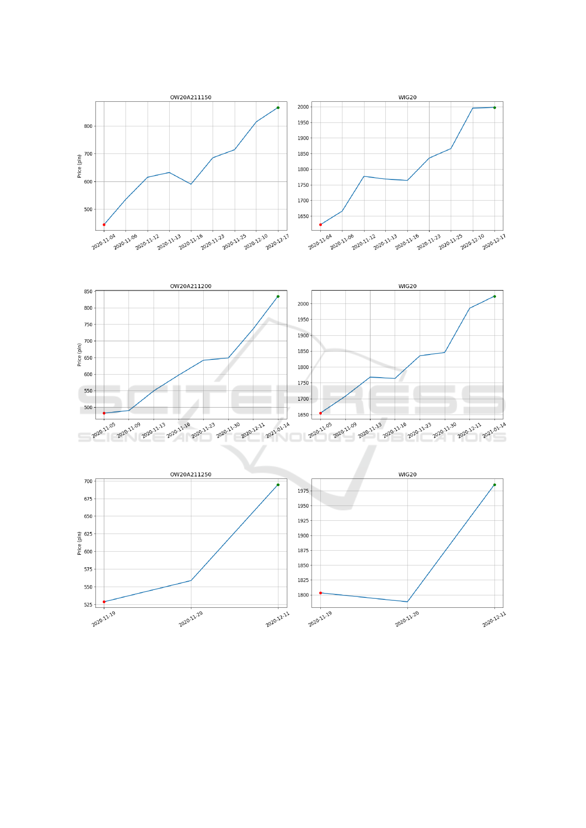
Figure 3: Historical data for OW20A211150 option (left) and WIG20 asset (right).
Figure 4: Historical data for OW20A211200 option (left) and WIG20 asset(right).
Figure 5: Historical data for OW20A211250 option (left) and WIG20 asset (right).
option valuation and it implies zero value of the pa-
rameter β. For theses options the non-linear model
is equivalent to the linear one. The option prices ob-
tained from the non-linear model were burdened with
the relative error less than 0.5% with respect to the
options market values. For options OW20A212050
and OW20A212075 the absolute error is equal to zero
while the realtive error is not available.
COMPLEXIS 2022 - 7th International Conference on Complexity, Future Information Systems and Risk
32

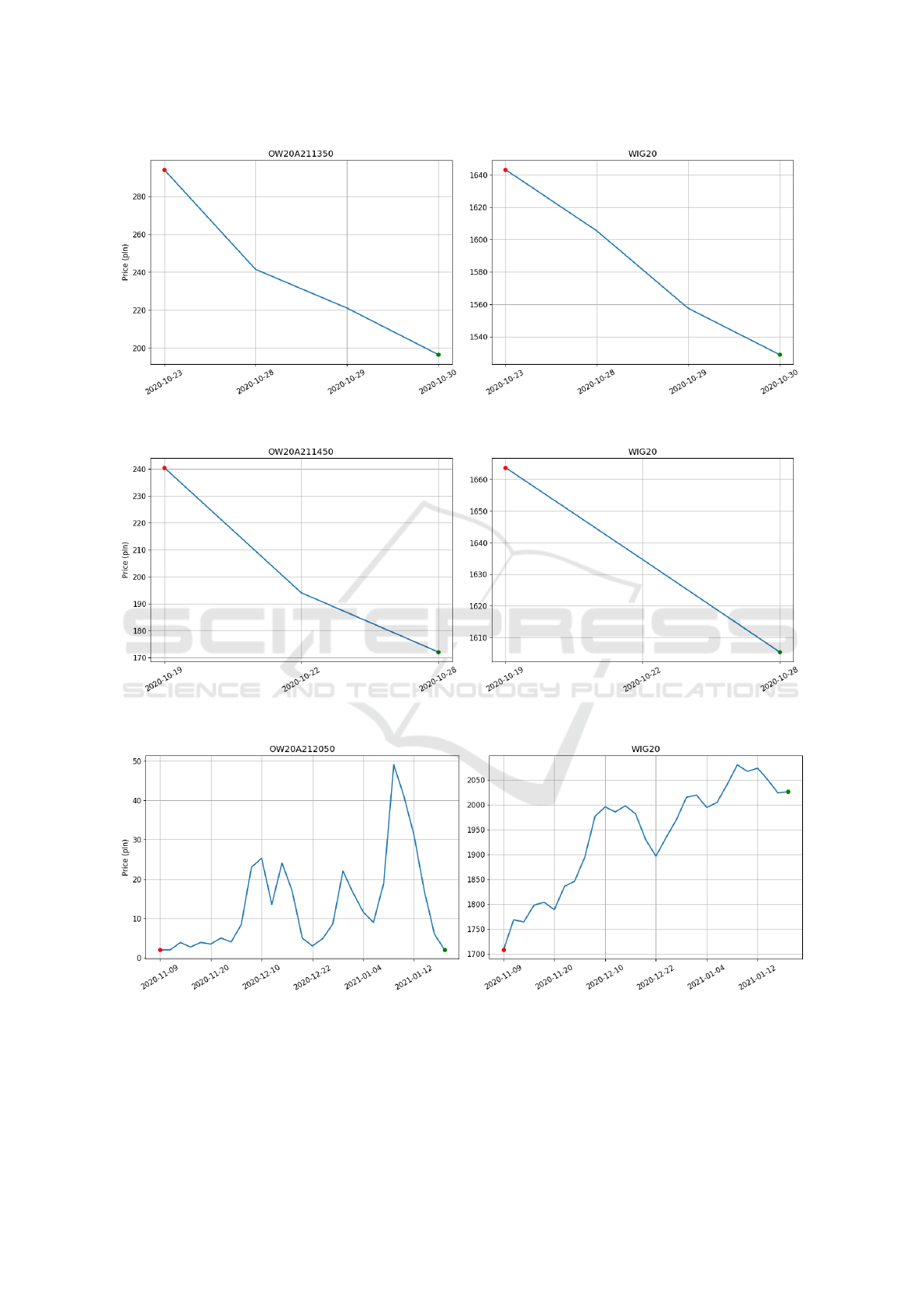
Figure 6: Historical data for OW20A211350 option (left) and WIG20 asset (right).
Figure 7: Historical data for OW20A211450 option (left) and WIG20 asset (right).
Figure 8: Historical data for OW20A212050 option (left) and WIG20 asset (right).
The proposed non-linear model provides much
more accurate results than linear model with the
volatility parameter σ taken from the market as asset
price volatility. The linear model can provide more
accurate results, but only under condition that param-
eter σ is calibrated. It is also interesting to observe
that in general, parameter β takes low values. We
have also calculated option price using linear Black-
Non-linear Black-Scholes Option Pricing Model based on Quantum Dynamics
33

Figure 9: Historical data for OW20A212075 option (left) and WIG20 asset (right).
Table 2: Numerical results for parameter β calibration and option calculation.
Option Beta V=S-K L (L-V)/V NL (NL-V)/V
OW20A211150 -0.00000782 847.910 473.644 -44.139826 % 847.568 -0.040334 %
OW20A211200 -0.00000557 823.830 456.909 -44.538460 % 823.195 -0.077079 %
OW20A211250 -0.00000775 735.510 554.243 -24.645076 % 735.886 0.051121 %
OW20A211350 0.00008887 178.780 293.599 64.223627 % 178.721 -0.033001 %
OW20A211450 0.00011914 155.430 214.107 37.751399 % 155.522 0.059191 %
OW20A212050 0.00000000 0.000 0.000 n/a 0.000 n/a
OW20A212075 0.00000000 0.000 0.000 n/a 0.000 n/a
Scholes formula for the given set of parameters. In the
case of option price predicted by this model is lower
than expected one, i.e. is underestimated option price,
then parameter β < 0. If the option price predicted by
linear Black-Scholes model is higher than expected,
i.e., overestimated option price, then parameter β > 0.
6 CONCLUSIONS
Quantum mechanics is describing the dynamics of
micro world. It was an inspiration to create a new
model describing option pricing using phenomeno-
logical approach. Extended non-linear Black-Scholes
model for option pricing has been proposed.The
model has been obtained by transforming into Eu-
clidean space non-linear Schr
¨
odinger equation. The
method of lines has been used to solve numerically
classical linear and the proposed non-linear Black-
Scholes models. Non-linear Black-Scholes model has
been also calibrated based on market data, including
historical volatility, risk-free rate, strike price and ex-
piration time for a given options based on WIG20 in-
dex stock and listed on Warsaw Stock Exchange. Cal-
ibration was performed using divide and conquer al-
gorithm to optimize the parameter β value.
The obtained results indicate that the proposed
non-linear model for option pricing is much more ac-
curate than the classical linear Black-Scholes model
and provides option prices differing only less than
0.5% with respect to their market prices. In con-
trary, linear Black-Scholes model with volatility σ
taken from the market provides very inaccurate re-
sults significantly different than market option prices.
The computational complexity of the model equals
O(nlog n) and is relatively low. The developed model
can be efficient calibrated in easy and efficient way.
Since the parameter β is fairly well defined the model
can be used for option forecasting. The proposed
model is being extended to deal with American or
Asian type options.
REFERENCES
Barles, G., Soner, H.N. (1998). Option pricing with trans-
action costs and a nonlinear Black-Scholes equation.
Financ. Stoch., 2:369-397.
Black, F., Scholes, M. (1973). The pricing of options and
corporate liabilities. Journal of Political Economy,
81:637-654.
Bollerslev, T. (1986). Generalized autoregressive condi-
tional heteroskedasticity. Journal of Econometrics,
31(3):307-327.
COMPLEXIS 2022 - 7th International Conference on Complexity, Future Information Systems and Risk
34

Bose, S. N. (1924). Plancks Gesetz und Lichtquantenhy-
pothese. Zeitschr. Phys. 26:178-181.
Clark, P.B. (1973). Uncertainty, exchange risk, and the level
of international trade. Economic Inquiry, 11(3):302-
313.
Debnath, L. (2005). Nonlinear Partial Differential Equa-
tions for Scientists and Engineers. Second Edition,
Birkh
¨
auser, Boston., p. 518. doi: 10.1007/b138648.
Einstein, A. (1925). Quantentheorie des einatomigen ide-
alen Gases 2,Sitzungsb. Preuss. Akad. Wissensch. 8:3-
14.
Einstein, A. (1924). Quantentheorie des einatomigen ide-
alen Gases, Sitzungsb. Preuss. Akad. Wissensch.
22:261-267.
El Hajaji, A., Hilal, K. (2015). Numerical method for
pricing governing American options under frac-
tional Black-Scholes model, Mathematical Theory
and Modeling. 5:112 - 124.
Engle, R.F. (1982). Autoregressive conditional het-
eroscedasticity with estimates of the variance of
United Kingdom Inflation. Econometrica, 50(4):987-
1007.
Fama, E. (1965). The behavior of stock market prices. J.
Bus., 105:34-105.
Hamilton, J.D. (1989). A new approach to the economic
analysis of nonstationary time series and the business
cycle, Econometrica, 57:357-384.
Haven, E. (2004). The wave-equivalent of the
Black–Scholes option price: an interpretation,
Physica A: Statistical Mechanics and its Applica-
tions, 344(1-2):142-145.
Hayashi, M., Ozawa, T. (2016). Well-posedness for a gen-
eralized derivative non-linear Schr
¨
odinger equation, J.
Differential Equations. 261:5424-5445.
Heston, S. L. (1993). A closed-form solution for options
with stochastic volatility with applications to bond
and currency options, Review of Financial Studies.
6(2):327-343.
Hull, J., White, A. (1987). The Pricing of Options on Assets
with Stochastic Volatilities. The Journal of Finance,
42:281-300.
Ivancevic, V. G. (2011). Adaptive Wave Models for Sophis-
ticated Option Pricing. Journal of Mathematical Fi-
nance, 1(3):41-49.
Ivancevic, V. (2010). Adaptive Wave Alternative for the
Black-Scholes option pricing model, Cogn. Comput.,
2:17-30.
Jankova, Z. (2018). Drawbacks and Limitations of Black-
Scholes Model for Options Pricing. Journal of Finan-
cial Studies and Research, 1-7.
Kutta, W. (1901). Beitrag zur naherungsweisen Integra-
tion totaler Differentialgleichungen, Z. Math. Phys.
46:434-453.
Kong, Q., Siauw, T., Bayen, A. (2020). Python Program-
ming and Numerical Methods, Academic Press.
Marquardt, R., Quack, M. (2020). Molecular Spectroscopy
and Quantum Dynamics. Elsevier Inc.
Merton, R. C. (1973). Theory of Rational Option Pricing.
The Bell Journal of Economics and Management Sci-
ence, 4(1):141-183.
De la Pe
˜
na, L., Cetto, A. M. and Vald
´
es-Hern
´
andez,
A. (2020) Connecting Two Stochastic Theories That
Lead to Quantum Mechanics, Frontiers in Physics. 1 -
8.
Peszek, R. (1995). PDE Models for Pricing Stocks
and Options With Memory Feedback. Ap-
plied Mathematical Finance, 2(4):211-224. doi:
10.1080/13504869500000011.
Rendleman, J.R., Bartter, J.B. (1979). Two-State Option
Pricing. Journal of Finance, 24.
Rogel-Salazar, J. (2013). The Gross-Pitaevskii equation
and Bose-Einstein condensates. European Journal of
Physics. 34:247.
S
`
anchez Douqe, C., S
`
anchez Douqe, H., Gonzalez, J.R.
(2017). Approximate Analytical Solution for the
Black-Scholes Equation by Method of Lines, Contem-
porary Engineering Sciences, 33:1615-1629.
Schneider, G., Vecker, H. (2017). Nonlinear PDEs. A dy-
namical Approach. American Mathematical Society,
Providence, Rhode Island.
Smoluchowski, M. (1906). Zur kinetischen Theorie der
Brownschen Molekularbewegung und der Suspensio-
nen. Annalen der Physik, 21(14):756-780.
Townsend, J. S. (2012). A Modern Approach to Quantum
Mechanics. University Science Books, 247-272.
Vukovic, O. (2015) On the Interconnectedness of
Schrodinger and Black-Scholes Equation. Journal of
Applied Mathematics and Physics, 3:1108-1113.
Weinan, E., Tiejun, Li, Vanden-Eijden, E. (2019). Applied
Stochastic Analysis., American Mathematical Society,
Providence, Rhode Island.
Wr
´
oblewski, M. (2017). Nonlinear Schr
¨
odinger approach to
European option pricin. Open Physics. 15:280-291.
Wr
´
oblewski, M. (2013). Quantum physics methods in share
option valuation, Technical Transactions Automatic
Control 2-AC/2013:23-40.
Non-linear Black-Scholes Option Pricing Model based on Quantum Dynamics
35