Deep Semantic and Strutural Features Learning based on Graph for

Just-in-Time Defect Prediction

Abir M’baya

and Nejib Moalla

Universite Lumiere Lyon 2, DISP Laboratory, 160 Boulervard de Universite, 69500, Bron, France

Keywords:

Just-in-Time Defect Prediction, Semantic Features, Deep Learning, DGCNN, Code Property Graph.

Abstract:

Change-level defect prediction which is also known as just-in-time defect prediction, will not only improve

the software quality and reduce costs, but also give more accurate and earlier feedback to developers than tra-

ditional ﬁle-level defect prediction. To build just-in-time defect prediction models, most existing approaches

focused on using manually traditional features (metrics of code change), and exploited different machine

learning. However, those approaches fail to capture the semantic differences between code changes and the

dependency information within programs; and consequently do not cover all types of bugs. Such information

has an important role to play in improving the accuracy of the defect prediction model. In this paper, to bridge

this research gap, we propose an end to end deep learning framework that extracts features from the code

change automatically. To this purpose, we present the code change by code property sub-graphs (CP-SG)

extracted from code property graphs (CPG) that merges existing concepts of classic program analysis, namely

abstract syntax tree (AST), control ﬂow graphs (CFG) and program dependence graphs (PDG). Then, we apply

a deep graph convolutional neural network (DGCNN) that takes as input the selected features. The experi-

mental results prove that our approach can signiﬁcantly improve the baseline method DBN-based features by

an average of 20.86 percentage points for within-project and 32.85 percentage points for cross-project.

1 INTRODUCTION

The inspection of the entire code source of software

applications is often challenging, and testing all units

is not practical. To ensure high software quality and

reduce costs, early prediction of defects is very nec-

essary. Software defect prediction is used to predict

whether a source code artifact contains defects or not

in the early stages of development.Just-in-time soft-

ware defect prediction (JIT-SDP) is practical as it re-

duces the risk of introducing new defects during the

commit and the code can be expected by developers

with limited effort.

Machine learning algorithms have been widely

used by the researchers to improve the accuracy of the

JIT-defect prediction models. They use as input tra-

ditional features captured manually from the source

code. Almost all existing works use process metrics

such as code entropy (D’Ambros et al., 2012), change

entropy (D’Ambros et al., 2010), etc. to quantify

many aspects of historical development archived in

https://orcid.org/0000-0002-2531-1978

https://orcid.org/0000-0003-4806-0320

software repositories (version control and bug track-

ing systems).

However, all the above-mentioned metrics do not

reveal the syntax and semantics of code change. Pre-

vious researches on the ﬁle-level defect prediction

have demonstrated that the syntax and the semantics

of the programs represented either by abstract syn-

tax tree (AST) or control ﬂow graph (CFG) are use-

ful for characterizing defects (Shippey et al., 2019;

Dam et al., 2018). A recent study on ﬁle-level, proved

that syntax and semantics are not enough to cover

several types of bugs, speciﬁcally the bugs related to

the dependencies (Meilong et al., 2020). They sug-

gested combining semantic and structural features to

improve the prediction accuracy.

Code change ﬁles with different dependencies be-

tween data can have the same semantics and syn-

tax. For example, we consider the motivating ex-

ample in ﬁgure 1. It is about an implementation of

a simple functionality in a human resources context

whose purpose is to compute the salary increase per-

centage. The value of the raise variable should be as-

signed to the display function. However, it is missing

in ﬁle1.java. Thus, it will never be displayed on the

128

M’baya, A. and Moalla, N.

Deep Semantic and Strutural Features Learning based on Graph for Just-in-Time Defect Prediction.

DOI: 10.5220/0011061800003176

In Proceedings of the 17th International Conference on Evaluation of Novel Approaches to Software Engineering (ENASE 2022), pages 128-137

ISBN: 978-989-758-568-5; ISSN: 2184-4895

users’ screen. This is obviously a logical bug, which

can happen in real cases just as it did at McDonald’s

From a technical point of view, the raise variable’s

value is assigned but never used, making it a dead as-

signment. Figure 1 depicts two Java ﬁles ﬁle1.java

and ﬁle2.java, both of them have the same syntax and

semantic. Thus, using traditional features to represent

these two code snippets such as metrics or AST have

identical feature vectors. However, dependency in-

formation is different. Features that can discriminate

such structural differences should have a great impact

on the improvement of prediction accuracy. Taking

the example in ﬁgure 1, features that ensure that any

variable assigned in the program has a dependency

relationship, and so it is used by another instruction

should meaningful. It is therefore important to high-

light the dependencies of data or of control in the pro-

gram. Such information may help to select expressive

features for defect prediction.

Deep learning is one of the most meaningful sub-

ﬁeld of machine learning. It proved its efﬁciency in

developing more accurate defect prediction models by

leveraging selected expressive features automatically

generated from the source code and then these fea-

tures are used to train and construct the defect predic-

tion models (Hoang et al., 2019; Wang et al., 2018).

Speciﬁcally, we use a deep graph convolutional neu-

ral network (DGCNN) to learn defect features ex-

tracted from the code change. To use DGCNN, we

extract meaningful features by representing the code

change by a suitable representation called code prop-

erty graph (see details in the next section) that com-

bines the three classic program representations AST,

CFG, and PDG.

In this paper, we examine our deep semantic

and structural features learning based on graphs for

change-level defect prediction tasks. This work en-

ables us to compare our proposed approach with ex-

isting JIT-DP techniques.

Prior defect prediction studies are carried out in

one or two settings, i.e. cross-project defect predic-

tion (Xia et al., 2016a; Nam et al., 2013) and within-

project defect prediction (Jiang et al., 2013; Xia et al.,

2016b). Therefore, we analyze the effectiveness of

our approach using different evaluation measures un-

der different evaluation scenarios in the two settings

as well. We ﬁrst apply the non-effort-aware evalua-

tion scenario using Precision, Recall, and F1 metrics

that are commonly used in numerous studies (Nam

et al., 2013; Wang et al., 2016). Also, we conduct

an effort-aware evaluation scenario to examine the

practical aspect of our approach by applying PofB20

(Mende and Koschke, 2010).

https://bit.ly/32NzILG

In summary, the main contributions of this paper

are:

• Exploring deeply the code change by proposing a

suitable representation called code property graph

(CPG) inspired from a recent work (Yamaguchi

et al., 2014). CPG is used to detect vulnerabil-

ities in source code in (Yamaguchi et al., 2014)

but in this work, it allows expressing patterns

linked to defective code including syntax, seman-

tic, and dependency information. Experimentally,

exploiting code property graphs in the ﬁeld of de-

fect prediction proves its effectiveness in develop-

ing high-performance classiﬁers.

• Demonstrating the inability of the traditional fea-

tures in automatically extracting different types of

bugs and especially those which are related to the

dependencies from source code changes.

• Proposing an end-to-end prediction model on

change- level to automatically learn graph-based

expressive features that are fed to the multi-view

multi-layer convolutional network

• An extensive evaluation under both the non-effort-

aware and effort-aware scenarios; performed on

four open source java projects demonstrates the

empirical strengths of our model for defect pre-

diction and shows that our approach achieves a

signiﬁcant improvement for within- project defect

prediction and cross-project defect prediction.

The remainder of this paper is structured as fol-

lows: Section background reviews the representation

of code ’Code Property Graph’. Section III repre-

sents the related work. Then we provide details of our

proposed step-by-step approach in section IV. Section

V analyses the experimental results and evaluates the

performance of our approach. Section VI represents

threats to our work. We conclude the paper and sum-

marize the future outlines in section VII.

2 BACKGROUND

2.1 Code Property Graph

Software defects are deeply hidden in programs’ se-

mantics. It is therefore required to exploit the source

code and devise a suitable representation of the code

that allows us to mine large amounts of code and ex-

press patterns linked to defective code. As a solution,

we propose a powerful representation of code in by

leveraging a joint representation of a program’s syn-

tax, control ﬂow, and data ﬂow called code property

graph (CPG). The key insight underlying this repre-

sentation is to explore deeply the programs and reveal

Deep Semantic and Strutural Features Learning based on Graph for Just-in-Time Defect Prediction

129

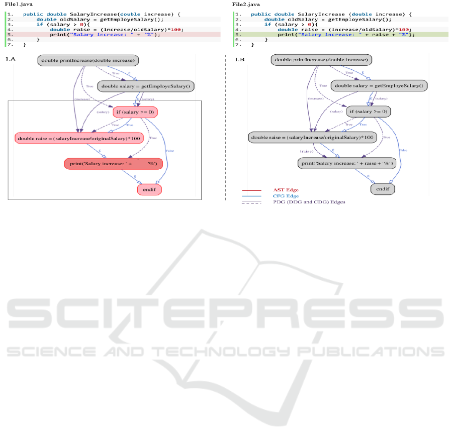
Figure 1: A motivating example. The variable increase corresponds to the difference between the new salary and the old

salary. The raise percentage which is deﬁned by the variable raise is computed in line 4 in both ﬁle1.java and ﬁle2.java.

several types of bugs in the source code. CPG is a

single representation that merges the three basic con-

cepts of program analysis including abstract syntax

tree (AST), control ﬂow graph (CFG), and program

dependency graph (PDG). Such a structure combines

the strengths of each representation and includes sev-

eral kinds of information at once. Hence, ASTs clar-

ify the structural information of the program, but nei-

ther captures the control ﬂow of programs nor the

intra-procedural dependencies. Therefore, they may

not determine many types of defects in programs.

CFGs addresses AST constraints, however, they fail

to clarify the dependencies among different program

entities within each method, even though the fact that

many bugs are directly related to the data ﬂow in-

formation and the relationship between executed in-

structions. Many researchers established a clear link

between the dependencies and appearances of several

bugs (Zimmermann and Nagappan, 2008; Li et al.,

2019). PDGs provide indications of the connectiv-

ity inside each method of the software. They clar-

ify data and control dependence between instructions

in a program. Without such interactions, software

will not be able to perform its required tasks and this

can eventually be a major contributor to the appear-

ance of bugs and to the difﬁculty in maintaining the

software. To sum up, CPG highlights different as-

pects of the program involving the syntactic, seman-

tic, and dependency information, by combining three

helpful program analysis and none can fully replace

the others. To achieve this, we drew inspiration from

a recent work (Yamaguchi et al., 2014) and use the

concept of property graph. The authors of the pa-

per (Yamaguchi et al., 2014) combine the three rep-

resentations for vulnerability detection in source code

which is different from ours, we combine those dif-

ferent in order to maximize the detection of differ-

ent types of defect features directly from the source

code.As the AST is the only one of the three represen-

tations which includes additional nodes, statements

and expressions serve therefore as transition points

from one representation to another. We can thus in-

corporate CFG and PDG into AST through the state-

ments and expressions. Each node is assigned by a

property key and its corresponding set of property val-

ues such as the key code and its property values (for-

statement, while-statement, if-statement, etc.) and the

key-property line and the corresponding property val-

ues (line-number, etc.) that indicates where the code

can be found. For example to link the AST and CFG

we get the property of each node of CFG and we

search in AST the nodes that have the same property

value as well as the same line number of code. Then,

we add the edges of CFG in AST between the two

nodes (source node and target node). Figure 2 repre-

sents a sample code and its corresponding AST, CFG,

PDG, and CPG. The property values of the node cor-

responding to the statement if (amount ¿ 0) are IF-

Statement and 3. In the AST, we add the edges (in-

coming edges and out-going edges) of CFG and PDG.

Same process to merge the AST and PDG to construct

the code property graph detailed in the ﬁgure2. We re-

fer to the paper (Yamaguchi et al., 2014) for more de-

tails how to model the three graphs as property graphs

and construct the code property graph by using the

same contextual-properties.

ENASE 2022 - 17th International Conference on Evaluation of Novel Approaches to Software Engineering

130

3 RELATED WORK

3.1 Just-in-Time Defect Prediction

Most of the existing studies represent the code by

designing traditional metrics (process metrics, code

metrics,etc.) to extract code properties and build the

predictive model by applying machine learning algo-

rithms. Kim et al. used text-based metrics accumu-

lated from change logs, ﬁle names, and the identiﬁers

in deleted and added source code; then applied sup-

port vector machine SVM to predict whether a change

contains bugs or not (Kim et al., 2008).

Kamei et al (Kamei et al., 2012) selected 14

change metrics of different categories such as size,

history, experience, etc. and developed logistic re-

gression models to predict commits as buggy or not.

Later on, they extended their work and evaluated the

feasibility of their proposed method in a cross-project

context (Kamei et al., 2010). Moser et al. (Moser

et al., 2008) used different history metrics such as

the number of revisions, ages of ﬁles, and past ﬁxes

to predict defects. Yang et al. (Yang et al., 2015),

Barnett et al. (Barnett et al., 2016), and Rahman et

al. (Rahman et al., 2011) applied another alternative

approach to increase JIT-DP accuracy such as deep

learning, cashed history, and textual analysis. Wang

et al. (Wang et al., 2018) proposed DBN-based se-

mantic features and examined the performance of the

built models on change- level and ﬁle-level for both

cross and within defect prediction tasks.

All the above mentioned traditional features are

manually encoded and still ignore the structural and

semantic information of programs as well as the de-

pendencies between entities within methods.

3.2 Deep Learning in Software

Engineering

Deep learning techniques have been widely applied

in defect prediction (Ferreira et al., 2019). Yang et

al. (Yang et al., 2015) leveraged DBN from a set of

change metrics such as code deleted, modiﬁed direc-

tories, metrics related to developers ’experience, etc.

to predict a commit as buggy or not. Wang et al (Wang

et al., 2018) generated semantic features based on the

program’s AST and used DBN to automatically learn

advanced features. Then, they performed defect pre-

diction by applying a regression classiﬁer. Li et al.

(Li et al., 2017) applied convolutional neural network

CNN to generate expressive features with structural

and semantic information. They combine traditional

features with CNN-learned-features to improve the

ﬁle-level prediction accuracy. Dam et al. (Dam et al.,

2018) rely on the usage of a tree-structured LSTM

network based on the intermediate representation of

the source code AST. The experiments conﬁrmed the

effectiveness of the proposed method on ﬁle- level for

both within and cross-project.

4 APPROACH

In this section, we establish our proposed software de-

fect prediction process relying on the code property

graph, providing granular detail and a thorough un-

derstanding of data ﬂows. The overall framework is

depicted in ﬁgure 3. The framework is mainly com-

posed of ﬁve steps: 1) labeling and data extraction, 2)

data-preprocessing: feature extraction based on code

property graph 3) encoding, 4) learning and evalua-

tion, and 5) prediction. We outline the details of each

step in the overall framework in the following sub-

sections.

4.1 Labeling and Data Extraction

In this step, we give a label to each change as buggy or

clean and identify the bug-introducing changes based

on version control data (e.g. Git) and bug report

stored in an issue tracking system (e.g. JIRA) of a

project by applying SZZ algorithm (Fan et al., 2019).

4.2 Feature Extraction

The objective of this phase is to represent the code

change by a suitable representation and extract mean-

ingful features from previous commits. Since the syn-

tax information of change data is often incomplete,

building AST, CFG, and PDG for these changes di-

rectly from code is challenging. Therefore, the learn-

ing is carried out with sub-graphs of code property

graphs that represent the code change. To do this, we

ﬁrstly parse the source code of each ﬁle into CPG by

merging AST, CFG, and PDG as outlined in the code

property graph section. Then, we extract the code

property sub-graph from the code property graph,

which represents the code changes. To do this, we

select only the nodes which are made from changed

lines and all their direct neighbours as well as all the

corresponding edges. Figure 1.A represents the code

property graph corresponding to the sample code in

ﬁle1.java. The nodes of the sub-graph are coloured in

red. The nodes in dark red represent the code change

while the nodes in light red represent the direct neigh-

bours. The code property sub-graphs are constructed

by following the steps below: 1) we identify ﬁrstly

all the lines that have been changed. For each ﬁle

Deep Semantic and Strutural Features Learning based on Graph for Just-in-Time Defect Prediction

131

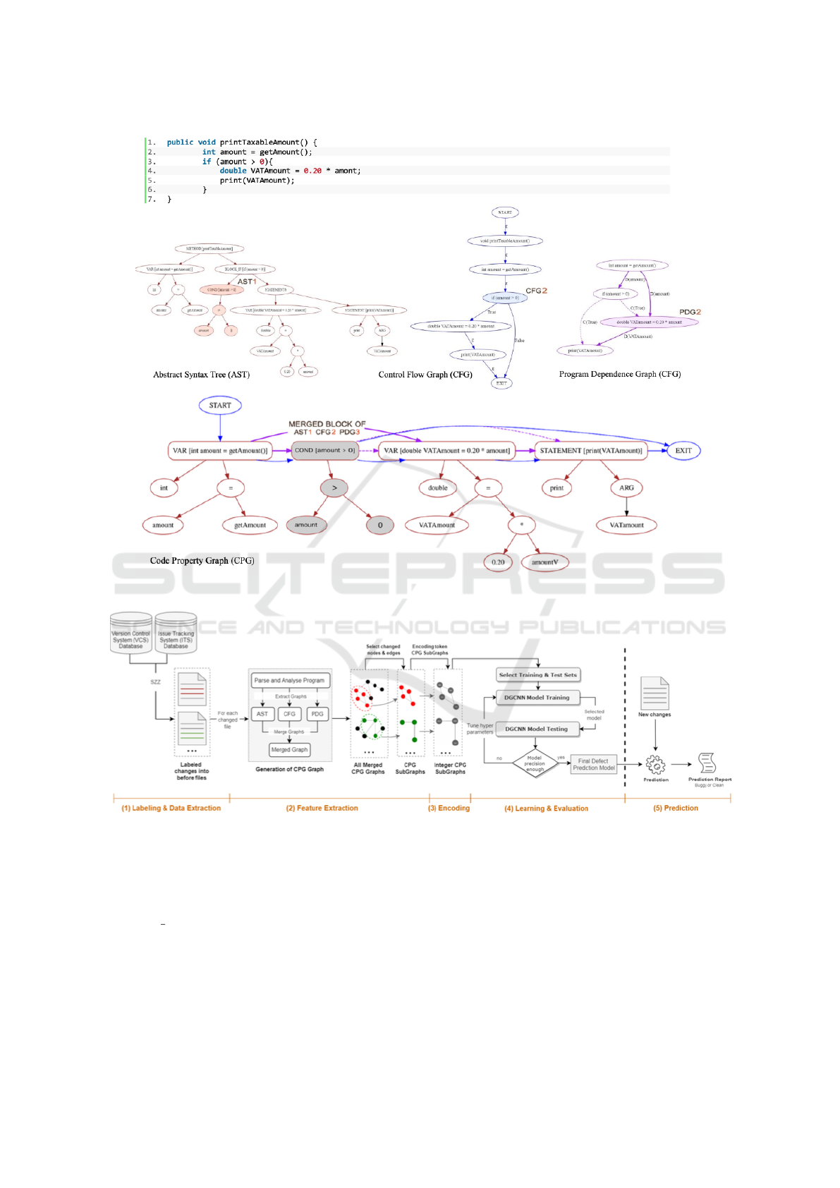
Figure 2: A code sample and its corresponding AST, CFG, PDG, and CPG.

Figure 3: The overall just-in-time defect prediction framework.

that represents the last version of the ﬁles before in-

troducing changes, we annotate all the modiﬁed or

deleted lines corresponding to their changed lines by

adding a comment with a speciﬁc format //[Unique-

Identiﬁer] T with T = M (modiﬁed), D (deleted).

Figure 4 depicts a sample of code change that intro-

duces a bug. As we can see in ﬁle2.java in ﬁgure 1,

line 5 was modiﬁed by adding the variable raise to ﬁx

the logic bug described above. Thus, we annotate the

line 5 in ﬁgure 4 by adding the speciﬁc comment and

the variable T takes the value M to indicate that this

line has been modiﬁed. 2) In the second step, we need

to store whether the nodes representing the CPG of

each ﬁle is making from a changed line or not. There-

fore, we assign the type T affected to the changed line

to its corresponding node in CPG. Taking the example

of the code sample in ﬁgure 1, the node correspond-

ing to the print () function is assigned by the character

M which is given as an annotation in the correspond-

ing line 5 as shown in ﬁgure 4. 3) Finally, we select

ENASE 2022 - 17th International Conference on Evaluation of Novel Approaches to Software Engineering

132

Figure 4: The identiﬁcation of change introducing bugs.

The unique identiﬁer is to separate the original comment

from the speciﬁc one, and the characters M and D represent

the modiﬁed line and deleted line respectively.

only the nodes having the type M or D and all their di-

rect neighbours as well as all the corresponding edges

to extract the code property sub-graph that represents

only the code change of the ﬁle.

4.3 Encoding

In this step, we encode the token sub-graphs to integer

sub-graphs by using a well-known method word2vect

(Mikolov et al., 2013) as the DGCNN takes only nu-

merical data. Furthermore, we equalize all the con-

verted integer vectors by adding O.

4.4 Employing the Deep Graph

Convolutional Neural Network

DGCNN

DGCNN is used in our proposed predictive system to

insert complex, high dimensional data integral in code

property sub-graphs for efﬁcient classiﬁcation of de-

fects. There are three consecutive stages to be per-

formed by the DGCNN based algorithms:Graph con-

volutionallayers, Sortpooling layer, and 3) the predic-

tion.

4.5 Building Classiﬁers and Performing

Defect Prediction

The classiﬁer can be built and trained by using their

features as well as their labels i.e. defective or clean,

and then the test data is used to analyze this classi-

ﬁer’s performance.

5 EXPERIMENTS AND RESULTS

In this section, we evaluate the effectiveness of our

proposed semantic and structural features based on

graphs and compare them with the state-of-the-art-

methods.Initially, the used standard datasets are pre-

sented and then the experiment setup. After this the

baseline techniques are presented and the evaluation

criteria for used performance are described. Finally,

research questions (RQ) are proposed and answered.

5.1 Dataset

We choose existing widely used Java datasets for eval-

uating change level defect prediction tasks (Xia et al.,

2016b), (Tan et al., 2015). This allows us to com-

pare our approach with existing just-in-time defect

prediction models on the same datasets and obtain a

process-safe evaluation. We select four Java open-

source Jackrabbit, Lucene; Jdt (from Eclipse), and

Eclipse platform. Table 1 shows the details about

these projects in terms of LOC and the number of

changes. We rely on the SZZ algorithm to label the

bug-ﬁxing changes of these projects.

5.2 Experiment Setup

1. Change-level Within-project Defect Prediction:

For each project listed in table 1, we used the

training data to construct the predictive model,

and apply it to the test data to analyse the

accuracy of the built model. According to the

authors of these papers (Kamei et al., 2012;

Kamei et al., 2016), change-level data are always

imbalanced. i.e. there are fewer buggy instances

than clean instances in the training data that can

introduce noise/bias and lead to a poor prediction

performance. For a fair comparison, we apply the

same settings as Tan’paper (Tan et al., 2015) to

overcome this issue. In this way, the training set

will be more balanced (Tan et al., 2015).

2. Change-level Cross-Project Defect Prediction:

To develop just-in-time defect prediction models

for the projects which have not enough training

data, the state-of-the-art proposes change-level

cross projects. The objective of cross-project

methods is to train the predictive models by utiliz-

ing the data of existing projects, known as source

projects. After this, the trained models are used

for predicting the defects in new projects, known

as target projects.

5.3 Baseline Methods

The proposed approach is evaluated by comparing it

with the given baseline methods:

• DBN-based features (Wang et al., 2018): This

method performs the DBN algorithm.

• CBS+ (Huang et al., 2019): a simple super-

vised predictive model that leverages the idea of

both the supervised model (EALR) (Kamei et al.,

2012) and the unsupervised model (LT).

Deep Semantic and Strutural Features Learning based on Graph for Just-in-Time Defect Prediction

133

5.4 Performance Evaluation Criteria

To analyze the precision of the predictive models,

we used the non-effort-aware and the effort-aware

analysing metrics.

1. Non-effort-aware Evaluation: three performance

metrics were used that are commonly adopted by

the studies to analyze the models of defect predic-

tion. The measures include recall, accuracy, and

F1 score.

2. Effort-aware Evaluation: Under the effort-aware

scenario, we use the PofB20 metric (Jiang et al.,

2013) for identifying the accurate percentage of

defects observed by monitoring the ﬁrst 20% lines

of code.

5.5 Results

In this section we present the results of our experi-

ments which are designed to answer the following re-

search questions:

1. RQ1: Do structural and semantic features based

on graphs outperform the state-of-the-art baseline

for change-level within-project defect prediction?

(a) Non-effort-aware Evaluation: To address this

question, we need to compare it with the base-

line methods. As the code source of both

baselines are not available, we take the val-

ues from their experiment results provided in

their papers and we consider only Java datasets.

Thus, we compare our approach with DBN and

CBS+ on the available Java datasets (Jackrab-

bit, Lucene and JDT) and (JDT and Plateform)

respectively; and pick the available values of

DBN and CBS+. Table 2 shows the F1 results

of both of them. It can be observed that our

CPG- based features outperform signiﬁcantly

the baseline DBN based change features on av-

erage of 20.86 percentage points and CBS+ on

average of 34.1 percentage points.

(b) Effort-aware Evaluation: We further conducted

a new experiment for change-level within-

project defect prediction by computing the

PofB20 metric. In table 3, the PofB20 values

of the defect prediction models are displayed

with the CPG-based features as well as with

the baseline DBN-based features. The PofB20

score varies from 33 to 49 percentage points.

Compared to DBN, our approach achieves an

improvement on average of 11.8 percentage

points.

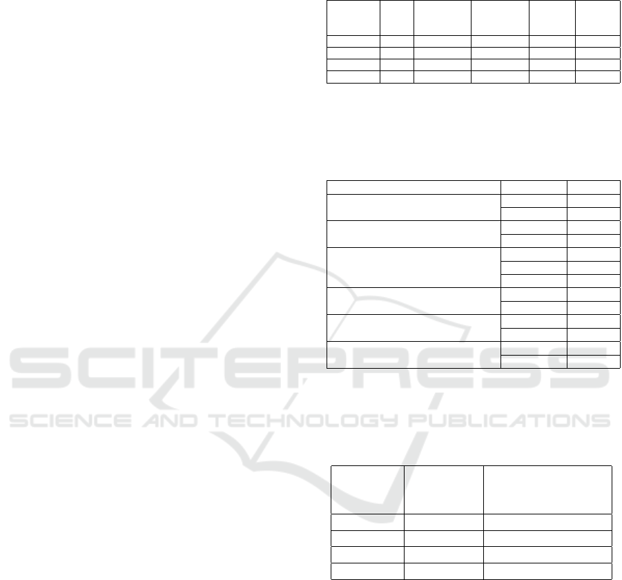
Table 1: Selected Java open-source Projects. LOC is the

number of lines of code. First Date is the date of the ﬁrst

commit of a project. last Date is the date of the last commit

of a project. changes is the number of changes.

Average

Projet LOC First Date Last Date Changes Buggy

rate (%)

JDT 1.5M 2001/06/05 2012/07/24 73K 20.5

Lucene 828K 2010/03/17 2013/01/16 76K 23.6

Jackrabbit 589K 2004/09/13 2013/01/14 61K 37.5

Platform 2001/20 2007/12 64K 25

Table 2: Selected Java open-source Projects for change-

level defect prediction. LOC is the number of lines of code.

First Date is the date of the ﬁrst commit of a project. last

Date is the date of the last commit of a project. changes is

the number of changes.

Project Approach F1 score

Jackrabbit

DBN 49.9

CPG-based 74.55

Lucene

DBN 39.7

CPG-based 61.55

JDT

CBS+ 32.9

DBN 41.4

CPG-based 57.48

Platform

CBS+ 35.1

CPG-based 78.72

Average (Jackrabbit, Lucene, JDT)

DBN 43.66

CPG-based 64.52

Average (JDT Platform)

CBS+ 34

CPG-based 68.1

Table 3: F1 score values of our CPG-based features

are compared with the baseline methods for change-level

within- project defect prediction . where the PofB20 are

calculated in percent and the highest pofb20 scores are pre-

sented in bold.

CPG-based

Project features DBN-based features

F1 F1

Lucene 33.3 28.1

Jackrabbit 33 27.9

JDT 49 23.8

Average 38.4 26.6

2. RQ2: Do structural and semantic features based

on graphs outperform the state-of-the-art baseline

for change-level cross-project defect prediction?

(a) Non-effort-aware Evaluation: To answer this

question, we compare our technique with the

baselines DBN-CPP (Wang et al., 2018) and

CBS+ (Huang et al., 2019). To conduct an un-

biased comparison, a similar approach as that

of Wang (Wang et al., 2018) was applied and

which is also very close to the CBS+. There-

fore, we select the data of the training set of

one run from a source project and the test set

of one run from a different project to prepare

ENASE 2022 - 17th International Conference on Evaluation of Novel Approaches to Software Engineering

134

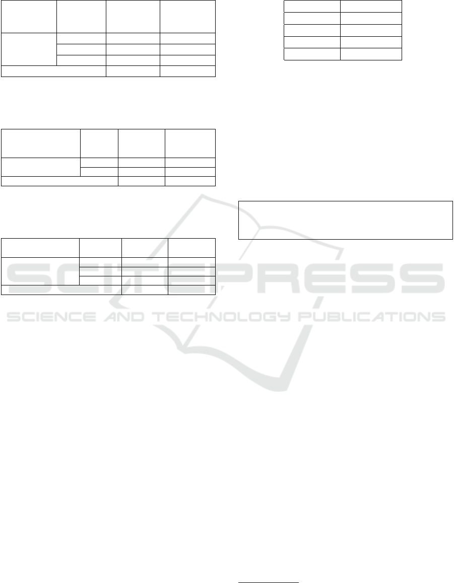
Table 4: F1 scores of our CPG-based features DBN-based

features for change-level cross-project defect prediction.

The F1 metrics are calculated in percent.

Source Target CPG-based DBN-based

Project project features features

F1 F1

All projects

Jackrabbit 72.69 44.4

Lacene 63.84 31.3

JDT 70.94 33.3

Average 69.15 36.3

Table 5: F1 scores of our CPG-based features and tradi-

tional features CBS+ for change-level cross-project defect

prediction. The F1 metrics are calculated in percent.

Source Target CPG-based CBS+-based

Project project features features

F1 F1

All projects

JDT 70.94 30.8

Platform 73.05 33.3

Average 71.99 32.05

Table 6: PofB20 scores our CPG-based features for change-

level cross-project defect prediction. the PofB20 metrics are

calculated in percent. The best values are in bold.

Source Target CPG-based DBN-based

Project project features features

All projects

Jackrabbit 42.0 19.3

Lacene 39.6 18.1

JDT 43.7 25.6

Average 41.7 21

the trial pairs. Table 4 presents the average F1

scores of the CPG based features with those of

DBN-CCP on three projects . The higher score

of F1 among them is displayed in bold. The re-

sults show that our approach signiﬁcantly im-

proves the average of F1 by 32.85 percentage

points for three projects. Moreover, we pro-

vide comparison results of CPG-based features

and CBS+ in table 5. Compared to CBS+ on

two projects, our approach achieves a better F1

score on average of 39.94 percentage points.

(b) Effort-aware Evaluation: During this evalua-

tion, we compute the PofB20 metric on change-

level cross- project defect prediction for our

proposed approach as well as the DBN-CPP.

Table 6 presents the scores of PofB20. For ev-

ery target project, we applied the other whole

source project as a training set and computed

the PofB20. As presented in Table 6, the scores

of PofB20 range from 39.6 to 43.7 % across the

experiments. We concluded that our approach

achieved a better PofB20 in every experiment.

This improvement depicts an average of 20.7

points.

3. RQ3: What are the time costs of our approach?

Table 7: Time cost of generating features involving the se-

mantics and the intra-procedural dependencies of the com-

mits source code.

Project time cost (s)

Lucene 49

Jackrabbit 58

JDT 80

Plateforme 75

This question leads to the study of the efﬁ-

ciency of our approach which is an important

indicator to assess whether or not the approach

is good enough.We measure therefore the time

taken for DGCNN-based features generation pro-

cess described in the sections 4.4 and 4.5. Ta-

ble 7 presents our method’ time cost on the four

datasets for generating features process. For every

project, the execution time automatically devel-

oped features based on DGCNN lies in the range

of 49 sec (Lucene) to the 80 sec (JDT).

Our CPG based semantic and structural features

learned automatically from the DGCNN is applica-

ble in practice.

6 THREATS TO VALIDITY

Threats involve potential errors that may have oc-

curred in the code implementation of our proposed

approach and study settings. Hence, to develop the

semantic feature with the dependency information,

we present the source code within the data struc-

ture known as CPG involving the AST, PDG, and

CFG. Since the original implementation of CPG is

not released, we have implemented a new CPG ver-

sion. Generally, we have followed the methods given

in previous studies (Yamaguchi et al., 2014), how-

ever, the newly developed CPG version may not re-

ﬂect each detail of the actual CPG. Therefore, we

have consulted with the writer of PROGEX

by email;

about the basic details of implementation and this was

the beginning of our framework implementation. We

are conﬁdent that the CPG implementation is quite

close to the original CPG, because the PROGEX in-

cludes the basic features which were useful for us to

implement the merge of graphs.

Moreover, we don’t possess the basic source code

to copy the techniques of (Wang et al., 2018; Huang

et al., 2019), therefore we have allowed ourselves to

consider the results they gave in their papers. We have

followed the same experiment settings just as it is ap-

plied in (Wang et al., 2018) in carrying out a compar-

https://github.com/ghaffarian/progex

Deep Semantic and Strutural Features Learning based on Graph for Just-in-Time Defect Prediction

135

ison with our approach. To realize a supplementary

comparison., we retrieved the results of (Huang et al.,

2019).

6.1 External Validity

Actually, our approach can be evaluated only on Java

open source projects. So, we conducted our exper-

iment only on four Java open-source projects that

have extensively been used in previous studies. This

can inﬂuence the generalizability of our results. To

mitigate this threat, further studies are required to

analyze our approach even to more datasets from

other types of projects whether proprietary software

or commercial one written in other programming lan-

guages. Other threats are related to the suitability

of our performance metrics to evaluate our JIT-DP

model. However, we use F1 and PofB20 which are

applied by past software engineering studies to anal-

yse various prediction techniques (noa, 2020; Xuan

et al., 2015).

7 CONCLUSION AND FUTURE

WORKS

This paper proposes an end-to-end deep learning

framework for just-in-time defect prediction to au-

tomatically learn expressive features from the set

of code changes.We conduct evaluations on four

open-source projects.The experiment results proved

that our approach improves signiﬁcantly the exist-

ing work DBN- based features and CBS+ on average

of 20.86 and 34.1 in F1, respectively in the task of

within-project defect prediction. Besides, it improves

the cross-defect prediction technique DBN-CPP and

CBS+ on average of 32.85 and 39.95 respectively in

F1. Also, our approach can outperform it under the

effort-aware evaluation context.

In the future, we would like to extend our eval-

uation to other open source and commercial projects

in order to reduce the threats to external validity. In

addition, we plan to make our framework applica-

ble to other open-source projects written in differ-

ent languages besides Java language, such as Python,

C/C++, etc.

REFERENCES

(2020). Multi-objective Cross-Project Defect Prediction -

IEEE Conference Publication.

Barnett, J. G., Gathuru, C. K., Soldano, L. S., and McIn-

tosh, S. (2016). The relationship between commit

message detail and defect proneness in java projects

on github. In 2016 IEEE/ACM 13th Working Confer-

ence on Mining Software Repositories (MSR), pages

496–499. IEEE.

Dam, H. K., Pham, T., Ng, S. W., Tran, T., Grundy,

J., Ghose, A., Kim, T., and Kim, C.-J. (2018). A

deep tree-based model for software defect prediction.

arXiv:1802.00921 [cs]. arXiv: 1802.00921.

D’Ambros, M., Lanza, M., and Robbes, R. (2010). An ex-

tensive comparison of bug prediction approaches. In

2010 7th IEEE Working Conference on Mining Soft-

ware Repositories (MSR 2010), pages 31–41. IEEE.

D’Ambros, M., Lanza, M., and Robbes, R. (2012). Evaluat-

ing defect prediction approaches: a benchmark and an

extensive comparison. Empirical Software Engineer-

ing, 17(4):531–577. Publisher: Springer.

Fan, Y., Xia, X., da Costa, D. A., Lo, D., Hassan, A. E., and

Li, S. (2019). The Impact of Changes Mislabeled by

SZZ on Just-in-Time Defect Prediction. IEEE Trans-

actions on Software Engineering.

Ferreira, F., Silva, L. L., and Valente, M. T. (2019). Soft-

ware Engineering Meets Deep Learning: A Literature

Review. arXiv preprint arXiv:1909.11436.

Hoang, T., Khanh Dam, H., Kamei, Y., Lo, D., and

Ubayashi, N. (2019). DeepJIT: An End-to-End Deep

Learning Framework for Just-in-Time Defect Predic-

tion. In 2019 IEEE/ACM 16th International Confer-

ence on Mining Software Repositories (MSR), pages

34–45.

Huang, Q., Xia, X., and Lo, D. (2019). Revisiting super-

vised and unsupervised models for effort-aware just-

in-time defect prediction. Empirical Software Engi-

neering, 24(5):2823–2862.

Jiang, T., Tan, L., and Kim, S. (2013). Personalized de-

fect prediction. In 2013 28th IEEE/ACM Interna-

tional Conference on Automated Software Engineer-

ing (ASE), pages 279–289. Ieee.

Kamei, Y., Fukushima, T., McIntosh, S., Yamashita,

K., Ubayashi, N., and Hassan, A. E. (2016).

Studying just-in-time defect prediction using cross-

project models. Empirical Software Engineering,

21(5):2072–2106.

Kamei, Y., Matsumoto, S., Monden, A., Matsumoto, K.-i.,

Adams, B., and Hassan, A. E. (2010). Revisiting com-

mon bug prediction ﬁndings using effort-aware mod-

els. In 2010 IEEE International Conference on Soft-

ware Maintenance, pages 1–10. IEEE.

Kamei, Y., Shihab, E., Adams, B., Hassan, A. E., Mockus,

A., Sinha, A., and Ubayashi, N. (2012). A large-

scale empirical study of just-in-time quality assur-

ance. IEEE Transactions on Software Engineering,

39(6):757–773. Publisher: IEEE.

Kim, S., Whitehead Jr, E. J., and Zhang, Y. (2008). Classi-

fying software changes: Clean or buggy? IEEE Trans-

actions on Software Engineering, 34(2):181–196.

Li, J., He, P., Zhu, J., and Lyu, M. R. (2017). Software

defect prediction via convolutional neural network.

In 2017 IEEE International Conference on Software

Quality, Reliability and Security (QRS), pages 318–

328. IEEE.

ENASE 2022 - 17th International Conference on Evaluation of Novel Approaches to Software Engineering

136

Li, Y., Wang, S., Nguyen, T. N., and Van Nguyen, S. (2019).

Improving bug detection via context-based code rep-

resentation learning and attention-based neural net-

works. Proceedings of the ACM on Programming

Languages, 3(OOPSLA):1–30.

Meilong, S., He, P., Xiao, H., Li, H., and Zeng, C. (2020).

An Approach to Semantic and Structural Features

Learning for Software Defect Prediction. Mathemat-

ical Problems in Engineering, 2020. Publisher: Hin-

dawi.

Mende, T. and Koschke, R. (2010). Effort-aware defect pre-

diction models. In 2010 14th European Conference

on Software Maintenance and Reengineering, pages

107–116. IEEE.

Mikolov, T., Chen, K., Corrado, G., and Dean, J. (2013).

Efﬁcient estimation of word representations in vector

space. arXiv preprint arXiv:1301.3781.

Moser, R., Pedrycz, W., and Succi, G. (2008). A compar-

ative analysis of the efﬁciency of change metrics and

static code attributes for defect prediction. In Proceed-

ings of the 30th international conference on Software

engineering, pages 181–190.

Nam, J., Pan, S. J., and Kim, S. (2013). Transfer defect

learning. In 2013 35th international conference on

software engineering (ICSE), pages 382–391. IEEE.

Rahman, F., Posnett, D., Hindle, A., Barr, E., and Devanbu,

P. (2011). BugCache for inspections: hit or miss? In

Proceedings of the 19th ACM SIGSOFT symposium

and the 13th European conference on Foundations of

software engineering, pages 322–331.

Shippey, T., Bowes, D., and Hall, T. (2019). Automatically

identifying code features for software defect predic-

tion: Using AST N-grams. Information and Software

Technology, 106:142–160.

Tan, M., Tan, L., Dara, S., and Mayeux, C. (2015).

Online defect prediction for imbalanced data. In

2015 IEEE/ACM 37th IEEE International Conference

on Software Engineering, volume 2, pages 99–108.

IEEE.

Wang, S., Liu, T., Nam, J., and Tan, L. (2018). Deep se-

mantic feature learning for software defect prediction.

IEEE Transactions on Software Engineering.

Wang, S., Liu, T., and Tan, L. (2016). Automatically learn-

ing semantic features for defect prediction. In 2016

IEEE/ACM 38th International Conference on Soft-

ware Engineering (ICSE), pages 297–308. IEEE.

Xia, X., Lo, D., Pan, S. J., Nagappan, N., and Wang, X.

(2016a). Hydra: Massively compositional model for

cross-project defect prediction. IEEE Transactions on

software Engineering, 42(10):977–998.

Xia, X., Lo, D., Wang, X., and Yang, X. (2016b). Collective

personalized change classiﬁcation with multiobjective

search. IEEE Transactions on Reliability, 65(4):1810–

1829.

Xuan, X., Lo, D., Xia, X., and Tian, Y. (2015). Evaluat-

ing defect prediction approaches using a massive set

of metrics: an empirical study. In Proceedings of the

30th Annual ACM Symposium on Applied Computing,

SAC ’15, pages 1644–1647, Salamanca, Spain. Asso-

ciation for Computing Machinery.

Yamaguchi, F., Golde, N., Arp, D., and Rieck, K. (2014).

Modeling and discovering vulnerabilities with code

property graphs. In 2014 IEEE Symposium on Secu-

rity and Privacy, pages 590–604. IEEE.

Yang, X., Lo, D., Xia, X., Zhang, Y., and Sun, J. (2015).

Deep learning for just-in-time defect prediction. In

2015 IEEE International Conference on Software

Quality, Reliability and Security, pages 17–26. IEEE.

Zimmermann, T. and Nagappan, N. (2008). Predicting de-

fects using network analysis on dependency graphs.

In Proceedings of the 30th international conference

on Software engineering, pages 531–540.

Deep Semantic and Strutural Features Learning based on Graph for Just-in-Time Defect Prediction

137