On the Use of Machine Learning for Predicting Defect Fix Time

Violations

Umit Kano

glu

1,2 a

, Can Dolas¸

1,2 b

and Hasan S

ozer

2 c

Turk Telekom, Ankara, Turkey

Ozyegin University, Istanbul, Turkey

Keywords:

Defect Fix Time Prediction, Bug Fix Time Prediction, Fix Time Violation, Classiﬁcation, Machine Learning,

Industrial Case Study.

Abstract:

Accurate prediction of defect ﬁx time is important for estimating and coordinating software maintenance ef-

forts. Likewise, it is useful to predict whether or not the initially estimated defect ﬁx time will be exceeded

during the maintenance process. We present an empirical evaluation on the use of machine learning for pre-

dicting defect ﬁx time violations. We conduct an industrial case study based on real projects from the telecom-

munications domain. We prepare a dataset with 69,000 defect reports regarding 293 projects being maintained

between 2015 and 2021. We employ 7 machine learning algorithms. We experiment with 3 subsets of 25

features derived from defects as well as the corresponding projects. Gradient boosted classiﬁers perform the

best by reaching up to 72% accuracy.

1 INTRODUCTION

Software projects are usually subject to delays (Bloch

et al., 2012) mainly as a result of ineffective risk man-

agement. An effective risk management requires the

ability and tool support (Choetkiertikul et al., 2015) to

predict the tasks that are at risk of being delayed. One

of these tasks is ﬁxing defects

. There have been re-

cent studies that exploit machine learning techniques

to estimate the ﬁx time of a software defect (Weiss

et al., 2007; Zhang et al., 2013; Lee et al., 2020; Ardi-

mento and Mele, 2020). These studies mainly employ

regression models to predict ﬁx time. In this study, we

employ classiﬁcation models to detect violations re-

garding these predictions or manual estimations. That

is, we aim at predicting whether or not the initially

estimated defect ﬁx time will be exceeded during the

maintenance process.

In this paper, we present an empirical evaluation

on the use of machine learning for predicting defect

ﬁx time violations. We conduct an industrial case

study based on real projects that are being maintained

https://orcid.org/0000-0001-8245-1355

https://orcid.org/0000-0003-0501-1625

https://orcid.org/0000-0002-2968-4763

We use the terms bug and defect interchangeably in the

rest of the paper.

by a telecommunications company. Telecommunica-

tions industry employs a wide range of software appli-

cations with a large customer volume and subscriber

transactions. These applications serve various pur-

poses such as customer relationship management, or-

der management, and workforce management. Tele-

Management Forum (TM Forum) (Mochalov et al.,

2019) has been recently introduced as a framework

that can host such applications that are developed

by telecommunications service providers around the

world.

We prepare a dataset that is composed of 69,000

bug reports regarding 293 projects being maintained

between 2015 and 2021. These reports are col-

lected from the Application Lifecyle Management

tool (K

ari

ainen and V

alim

aki, 2008) that is used in

the company. Another tool, namely the Enterprise

Architecture Management Application (Ernst et al.,

2006), is utilized for collecting information regarding

the projects associated with bug reports such as the

application type, programming language used and ar-

chitecture style adopted by the application. Some of

the collected data items such as keywords are directly

used as features for prediction. We also used Term

Frequency/Inverse Document Frequency (TF-IDF) to

derive additional features from textual descriptions.

We derive 25 features in total. We experiment with 3

different subsets of these features. In our experimen-

Kano

glu, Ü., Dola¸s, C. and Sözer, H.

On the Use of Machine Learning for Predicting Defect Fix Time Violations.

DOI: 10.5220/0011059900003176

In Proceedings of the 17th International Conference on Evaluation of Novel Approaches to Software Engineering (ENASE 2022), pages 119-127

ISBN: 978-989-758-568-5; ISSN: 2184-4895

119

tal setup, we employ 7 machine learning algorithms

including Random Forest, Multilayer Perceptron, Lo-

gistic Regression, K-Neighbors, Support Vector, Ex-

treme Gradient and Light Gradient Boosted classi-

ﬁers. Gradient boosted classiﬁers perform the best by

reaching up to 72% accuracy.

The remainder of this paper is organized as fol-

lows. We provide background information on the uti-

lized machine learning techniques in the next section.

In Section 3, the experimental setup is explained. We

present and discuss results in Section 4. Related pre-

vious studies are summarized in Section 5. We con-

clude the paper in Section 6.

2 BACKGROUND

In this section, we provide background information

regarding the techniques utilized in our study. Fix

time of a defect is estimated as soon as a defect is

opened. Our goal is to predict whether this estimated

time is going to be exceeded (i.e., violated) or not.

Hence, our goal is to solve a classiﬁcation problem

rather than a regression problem. In the following,

we ﬁrst explain TF-IDF, which is used for deriving

features from textual descriptions. Then, we explain

each of the classiﬁcation models employed in our

study.

2.1 TF-IDF and Feature Extraction

TF-IDF measures how important a word is to a docu-

ment. Term Frequency (TF) is obtained by multiply-

ing the number of times a term occurs in a document.

Inverse Document Frequency (IDF) is calculated as

the logarithm of the total number of documents di-

vided by the number of documents that include the

term (Parlar et al., 2016). In our study, keywords are

determined by considering the IDF scores of the terms

in all defect descriptions. By grouping these terms,

features are deﬁned from the sum of TF scores. For

example, “GUI” features are created by summing the

TF scores of terms such as button, combobox, menu

in the defect description. Thus, we employ TF-IDF

by calculating IDF for a set of keywords, before cal-

culating TF. First, the important terms are found by

considering their IDF scores. Then, the sum of the

TF scores of a set important terms are used as fea-

tures. These terms are identiﬁed within defect de-

scriptions and they are grouped according to relevant

project components.

2.2 Random Forest (RF)

RF classiﬁers employ a group of decision trees for

facilitating ensemble learning. Each decision tree as

part of the random forest provides a class prediction.

These predictions are collected from all the decision

trees and majority voting is applied to decide on the

ﬁnal outcome. RF classiﬁcation owes its success to

the combination of class predictions obtained from

many decision trees. These predictions have low or

no correlation at all. This is due to the use of bag-

ging and feature randomness. Bagging is applied for

ensuring that each decision tree uses a different train-

ing set although the size of the set is the same for all

the trees. Feature randomness leads to the use of dif-

ferent feature sets by different decision trees. RF is

known to be efﬁcient and effective when applied on

large datasets. However, it can be subject to overﬁt-

ting for such datasets (Yiu, 2021).

2.3 Multilayer Perceptron (MLP)

MLP model depends on the basic perceptron model

founded by Rosenblatt (Rosenblatt, 1958). A simple

perceptron model has a set of inputs. Each input is

associated with a weight. The model triggers an im-

pulse when the weighted sum of its inputs exceeds a

threshold value. This simple model has some draw-

backs. It can not imitate an XOR gate, for instance.

MLP is introduced to address this limitation. This

model employs a hidden layer between input and out-

put layers, where weighted sums are computed and

forwarded to the next layer. This process is known

as the feed forward approach. It requires the com-

pletion of a preliminary process called back propaga-

tion. This is a self learning process, where weights

are adjusted by calculating the mean squared errors

with respect to the expected output and propagating

these errors backward through the layers. This learn-

ing process continues until weights in all layers are

converged. MLP has the ability to cope with com-

plex non-linear datasets; however, it requires a high

amount of computational resources (Bento, 2021).

2.4 Logistic Regression (LR)

LR is a classiﬁcation algorithm based on a statistical

model used for estimating the probability of depen-

dent variables (Abhigyan, 2020). This method uses a

logit function to derive relationships between depen-

dent and independent variables. Then a sigmoid func-

tion (S-Curve) translates the derived relationships to

binary values to be used for prediction. It is a success-

ful method for predicting binary and linear scenarios

ENASE 2022 - 17th International Conference on Evaluation of Novel Approaches to Software Engineering

120

and for determining decision boundaries (Agrawal,

2021). This method is easy to implement and train

but it may lead to overﬁtting for large datasets. It is

computationally fast; however, it is successful mainly

for linearly correlated and separable, simple datasets.

It may fall short when there is not linearity between

independent variables.

2.5 K-Nearest Neighbors (KNN)

KNN is a supervised classiﬁcation algorithm that re-

lies on labelled datasets (Vatsal, 2021). KNN al-

gorithm labels data by measuring proximity among

neighbor data points to create correlations. K de-

notes the number of nearest neighbors with respect

to a speciﬁed unlabeled point. KNN measures the

distance of neighbors to that point. If K is set as

3, for instance, then the nearest 3 points proximity

can be measured and found by the chosen distance

metric type. Hereby, the mostly employed distance

metrics include Minkowsky, Euclidian and Manhat-

tan distance. The label of the point is decided by ma-

jority voting. The algorithm is simple and easy to im-

plement; however, the value of K must be optimized

to prevent overﬁtting. In addition, KNN needs high

computational power and storage capacity especially

when working on large datasets.

2.6 Support Vector Machines (SVM)

SVM is also a supervised algorithm commonly used

for classiﬁcation and regression problems (Yadav,

2018). The aim of the algorithm is basically to form

optimal hyperplanes that separate data points. Hy-

perplanes are formed by measuring their distances to

the data points, which are called as margins. The al-

gorithm adjusts hyperplanes to maximize these mar-

gins. Separations can be formed with lines in a two

dimensional space. However, hyperplanes are needed

in a three dimensional space. Optimal hyperplane di-

visions are robust against outliers and they are very

effective with separated classes. However, the algo-

rithm needs high computation power while working

with large datasets to form optimal hyperplanes (Ya-

dav, 2018).

2.7 Extreme Gradient Boosting (EGB)

EGB is an advanced machine learning algorithm that

is built upon decision trees and gradient decision ar-

chitecture. It exploits parallelization, tree pruning and

efﬁcient use of hardware. L1 (Lasso) and L2 (Ridge)

regularization are used for avoiding overﬁtting. This

approach concentrates on boosting weak learners by

handling missing data efﬁciently (Morde, 2019).

2.8 Light Gradient Boosting (LGB)

LGB is also a decision tree based high performance

algorithm for classiﬁcation problems. Main differ-

ence of this algorithm from EGB is that decision trees

grow horizontally instead of vertically. Unlike EGB,

LGB can handle large datasets and requires less mem-

ory space. However, LGB is inclined to be subject

to overﬁtting. Therefore, it is not suitable for small

datasets (Nitin, 2020).

3 EXPERIMENTAL SETUP

In this section, we explain our experimental setup in-

cluding our experimental objects, preparation of the

dataset, evaluation metrics and tuning of the machine

learning algorithms for classiﬁcation. Python pro-

gramming language is used in the study. Code de-

velopment is performed with Jupyter notebook. We

used the implementations of RF, MLP, LR, KNN,

SVM, EGB and LGB classiﬁcation algorithms from

the Scikit-Learn library (Hao and Ho, 2019).

3.1 Preparation of the Dataset

We utilized Application Lifecyle Manage-

ment (K

ari

ainen and V

alim

aki, 2008) and Enterprise

Architecture Management Application (Ernst et al.,

2006) tools to collect data regarding the reported

bugs and the corresponding projects, respectively.

Our dataset consists of 69,000 defects reported

for 293 projects from December 2015 to October

2021. We preprocessed the collected data to apply

basic corrections on lookup values, data format and

typographical errors. Then we derived 25 features as

listed in Table 1. Some of these features are directly

collected from the properties of the bug reports. For

instance, Day, Month, Season and Quarter features

are obtained from the issue date of the defect. Weekly

Defect is the weekly average number of defects that

is calculated based on the number of defects in the

last 1 year. Severity is a feature in ordinal scale, of

which value ranges between 1 (Low) and 5 (Urgent).

Defect resolution times vary according to severity

and the environment, in which it occurs. This time is

displayed in the Operational Level Agreement (OLA)

ﬁeld. Defects that are opened in September are

marked as Back to School. Defects that are opened

on Saturday and Sunday are marked as Weekend.

Environment feature identiﬁes whether the defect is

On the Use of Machine Learning for Predicting Defect Fix Time Violations

121

detected in a test or production environment. Main

Type indicates the particular environment, where

the defect is detected. Defect Type and Project

Phase identiﬁes the context and activity during

which the defect is detected. Telco Domain indicates

the application domain such as Mobile, Fixed and

Broadband. Application Type denotes the type of

application in nominal scale. Possible values for this

feature include Order Management (OM), Web Portal

(WP), Middleware (MW), Billing and Rating (BR),

Customer Relationship Management (CRM), Data

Warehouse (DW), Enterprise Resource Management

(ERP), Workforce Management (WFM), Collection

(COL), Messaging (MSG), Problem Management

(PM) and Document Management (DOC).

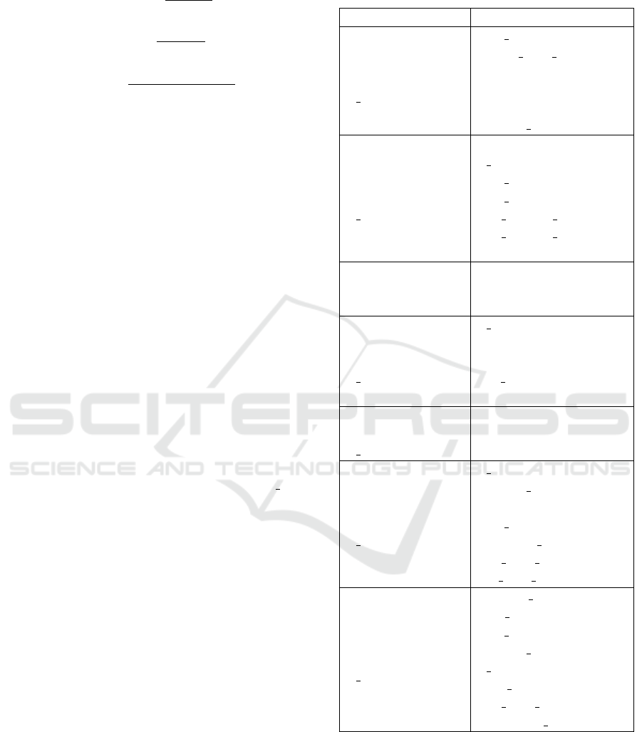
Table 1: The set of utilized features. Those feature that have

high importance are marked with *.

Features Description

Day* based on opening date

Month based on opening date

Season based on opening date

Quarter based on opening date

Weekly Defect* Weekly defect count

Severity* 1-Low, ... , 5-Urgent

OLA* Solution time

Back to School 0-No, 1-Yes

Weekend 0-No, 1-Yes

Main Type* 01 - TEST, 04 - PROD, ...

Environment TEST, PROD

Defect Type* Code, Analysis,...

Telco Domain* Mobile, Fixed, Broadband

App. Type* OM, WP, MW, BR, ...

Project Phase* Functional, Unknown,...

GUI* TF of buton, screen,...

Subscriber* TF of service, tariff, ...

Workﬂow TF of ﬂow, ...

Database TF of database, ﬁeld, ...

Workorder TF of workorder, ...

Order* TF of order, churn, ...

Device TF of cpe, device, ...

Integration TF of webservice, ...

Report TF of report, ...

Customer* TF of customer, account, ...

OLA Violation 0-Successful, 1-Violation

10 of features listed in Table 1 are derived from

textual descriptions using TF-IDF. First, we deter-

mined the mostly used terms in these descriptions

by calculating the corresponding IDF values. Sec-

ond, we performed a domain analysis using our in-

dustry experience to group these terms according to

their application context. The formed groups are

used as features, including GUI, Subscriber, Work-

ﬂow, Database, Workorder, Order, Device, Integra-

tion, Report, Customer. The value of each of these

features is set by summing up the TF scores of the

terms associated with the feature.

The last row of Table 1 lists OLA Violation. This

has to be predicted based on the 25 features. It is set

to 1 if the resolution time of the defect exceeds the

OLA time. It is set to 0, otherwise. We experiment

with 3 feature sets: i) All (A) contains all the 25 fea-

tures listed in Table 1; ii) High Importance (H) con-

tains those features that are considered as highly im-

portant and as such labelled with * in Table 1. These

features are determined as a result of the high impor-

tance feature selection with the random forest and lo-

gistic regression algorithms (Bonaccorso, 2017); iii)

Without TF-IDF (W) contains all the features expect

10 of them that are derived from textual descriptions

based on TF-IDF calculations. These are the ﬁrst 15

features listed in Table 1.

We created multiple models for prediction by

combining various machine learning techniques with

the 3 feature sets that are described above. We exper-

imented with combinations of different feature sets

and models to evaluate their effectiveness in predic-

tion. We describe the evaluation metrics in the fol-

lowing.

3.2 Evaluation Metrics

We expect our classiﬁer to provide a binary verdict:

the expected defect ﬁx time (i.e., OLA) is exceeded

(i.e., violated) or not. This verdict is considered a true

negative (TN), true positive (TP), false negative (FN),

or false positive (FP) as deﬁned below:

TN: There is no violation and the verdict is negative.

TP: There is violation and the verdict is positive.

FN: There is violation and the verdict is negative.

FP: There is no violation and the verdict is positive.

We evaluated the effectiveness of classiﬁers with

precision, recall, accuracy and F1 metrics that are

calculated based on the number of TN, TP, FN and

FP verdicts as listed in the following.

Accuracy =

|T P|+|T N|

|T P|+|FP|+|T N|+|FN|

(1)

ENASE 2022 - 17th International Conference on Evaluation of Novel Approaches to Software Engineering

122

Precision =

|T P|

|T P|+|FP|

(2)

Recall =

|T P|

|T P|+|FN|

(3)

F1 = 2 ×

Precision × Recall

Precision + Recall

(4)

These metrics are used for evaluating machine learn-

ing models, which are tuned and trained as described

in the following.

3.3 Model Tuning and Training

We used 7 different classiﬁers as described in Sec-

tion 2. Classiﬁers have different hyper parameters

and their performances differ according to parame-

ter settings. We experimented with various hyper pa-

rameter values by using all the features listed in Ta-

ble 1. We selected hyper parameters settings that lead

to the best recall values. These settings are obtained

by using randomized search and grid search (Bonac-

corso, 2017) as implemented in the Scikit-learn li-

brary. 360 different models are created by adopting

different combinations of hyper parameters for 7 dif-

ferent classiﬁers. Model performances are measured

with 10-fold cross validation (Bonaccorso, 2017). Ta-

ble 2 shows the values of hyper parameters that lead to

the best performance for each of the 7 algorithms. The

table also shows the employed hyper parameter opti-

mization method and the number of iterations (n iter)

used for each algorithm. We present and discuss the

results in the following section.

4 RESULTS & DISCUSSION

We created 7 models trained with 3 different feature

sets. Hence, we obtained 21 different models in total.

We present results obtained with these models in the

following. Then, we discuss these results and threats

to the validity of our evaluation.

Overall results are listed in Table 3 based on the

evaluation metrics described in Section 3.2. EGB

achieves the best accuracy (0.72), when all the fea-

tures are used except those derived from textual de-

scriptions. The best precision value (0.69) is obtained

with EGB and SVM, when only the features of high

importance are used or when we at least exclude those

derived from textual descriptions. LGB achives the

best F1 score (0.68) and the best recall value (0.72) re-

gardless of the feature set used for training the model.

In summary, LGB and EGB perform the best in terms

Table 2: Employed machine learning algorithms and their

hyper parameter settings.

Classiﬁer Hyper parameters

MLP

Randomized Search

n iter=50

max iter = 2000

hidden layer size = 100

activation = ‘tanh’

solver = ‘sgd’

alpha = 0.01

learning rate = ‘constant’

Randomized Search

n iter=50

criterion = ‘entropy’

n estimators = 800

max features = ‘auto’

max depth = 10

min samples split = 5

min samples leaf = 1

bootstrap = False

Grid Search

solver = ‘liblinear’

penalty = ‘l1’

C = 0.01

KNN

Randomized Search

n iter=50

n neighbors = 5

metric = ‘manhattan’

weights = ‘distance’

leaf size = 30

p = 2

SVM

Randomized Search

n iter=10

kernel = ‘rbf’

gamma = ‘scale’

C=1

EGB

Randomized Search

n iter=50

n estimators = 900

learning rate = 0.06

subsample = 0.9

max depth = 6

colsample bytree = 0.5

min child weight = 1

use

label encoder = False

LGB

Randomized Search

n iter=50

boosting type = ‘dart’

num leaves = 7

max depth = 79

learning rate = 0.228

n estimators = 766

class weight = ‘balanced’

min child samples = 10

importance type = ‘split’

of recall and precision, respectively. Detection of all

the violations is more important than an increased

number of false positive warnings for business pro-

cesses. That is, achieving high recall is relatively

more important than achieving high precision.

In general, we observe that the performance of

algorithms are not signiﬁcantly affected by the em-

On the Use of Machine Learning for Predicting Defect Fix Time Violations

123

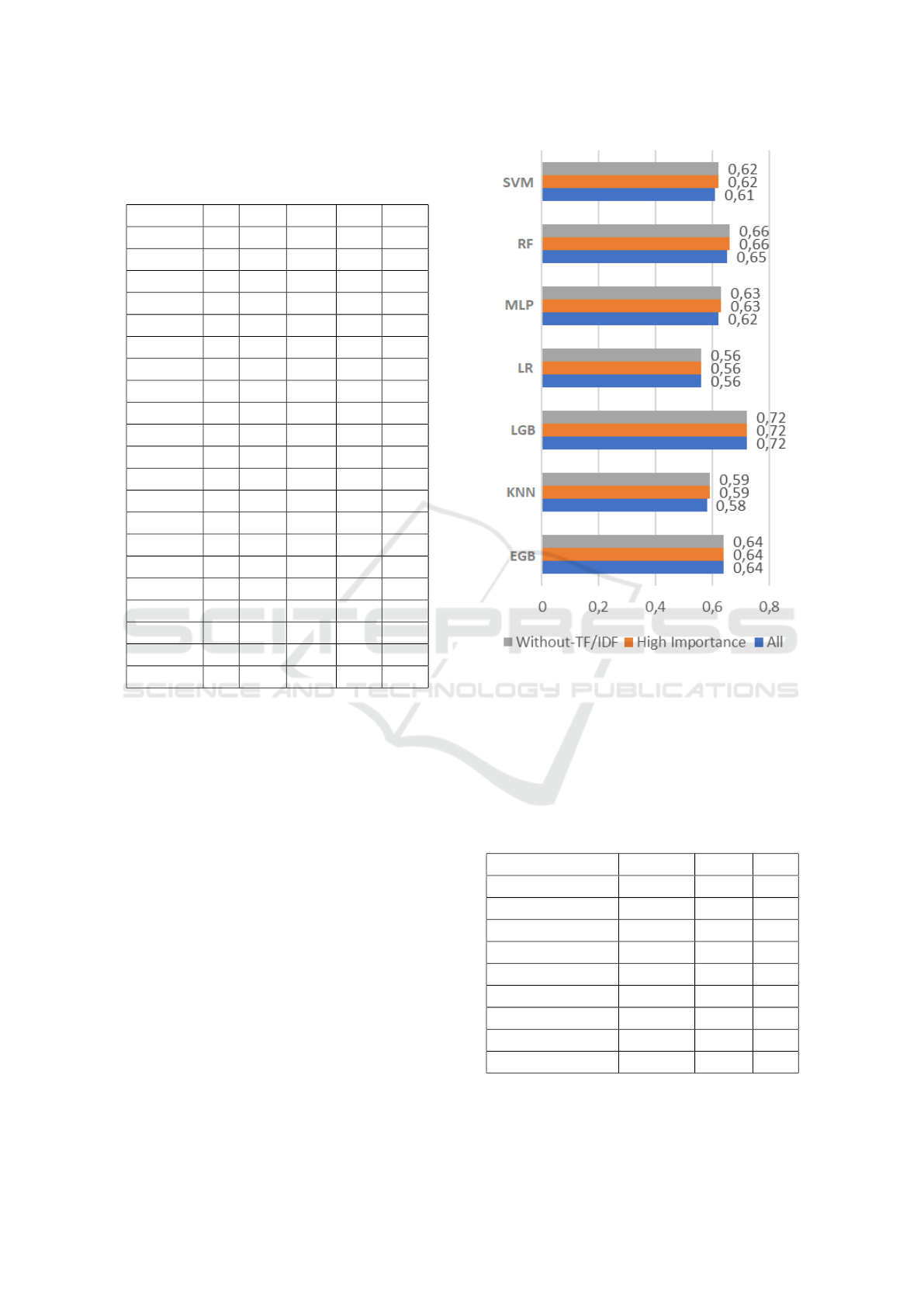
Table 3: Overall results regarding Accuracy (Acc.), Preci-

sion (Prec.), F1 score and Recall (Rec.) for 3 Feature Sets

(FS): A: All, H: High Importance, W: Without TF-IDF.

Classiﬁer FS Acc. Prec. F1 Rec.

LGB W 0.70 0.65 0.68 0.72

LGB A 0.70 0.65 0.68 0.72

LGB H 0.70 0.65 0.68 0.72

RF W 0.70 0.67 0.66 0.66

RF A 0.70 0.67 0.66 0.66

RF H 0.70 0.67 0.66 0.65

EGB W 0.71 0.69 0.66 0.64

EGB A 0.72 0.70 0.67 0.64

EGB H 0.72 0.70 0.67 0.64

MLP W 0.69 0.66 0.64 0.63

MLP A 0.69 0.66 0.64 0.63

MLP H 0.71 0.69 0.65 0.62

SVM W 0.71 0.69 0.65 0.62

SVM A 0.68 0.64 0.63 0.62

SVM H 0.70 0.69 0.64 0.61

KNN W 0.67 0.65 0.62 0.59

KNN A 0.67 0.65 0.62 0.59

KNN H 0.67 0.64 0.61 0.58

LR W 0.67 0.65 0.60 0.56

LR A 0.67 0.65 0.60 0.56

LR H 0.67 0.65 0.6 0.56

ployed set of features. In particular, LGB abd LR are

not affected at all. The difference for other classiﬁers

is mostly 0.01. The maximum difference is obtained

for SVM as 0.05, when all the features are used (0.64)

instead of only those with high importance (0.69).

Figure 1 shows the recall values obtained with the 7

algorithms for different feature sets. We see that the

results are mostly the same and the difference is never

larger than 0.01 for any of the algorithms.

Our evaluation metrics can be misleading for im-

balanced datasets. Therefore, we also calculated and

reported additional metrics for LGB and EGB, which

take the proportion of actual occurrences of classes

in the dataset into account. Table 4 shows the re-

sults, which are obtained with all the features. The

ﬁrst two rows listed for LGB and EGB of Table 4

show the performance of the algorithms for predict-

ing instances of two classes to be predicted: Viola-

tion and No violation. Macro average values are ob-

tained by ﬁrst calculating the corresponding metrics

for each class separately and then calculating their un-

weighted mean. Weighted average is also calculated

as the mean of measurements obtained for each class.

Figure 1: Recall values for 3 different feature sets.

However, the contribution of each class to the mean

value is weighted based on the number of instances of

the class taking place in the dataset. We see in Table 4

that there are no signiﬁcant differences or no differ-

ence at all between the macro and weighted average

scores.

Table 4: Results obtained with LGB and EGB for additional

metrics that reﬂect class imbalance.

LGB Precision Recall F1

No violation 0.75 0.69 0.72

Violation 0.65 0.72 0.68

Macro Average 0.70 0.70 0.70

Weighted Average 0.71 0.70 0.70

EGB Precision Recall F1

No violation 0.73 0.78 0.76

Violation 0.70 0.64 0.67

Macro Average 0.72 0.71 0.71

Weighted Average 0.72 0.72 0.72

Results obtained with LGB for 3 different feature

sets are depicted in Figure 2 in the form of confusion

ENASE 2022 - 17th International Conference on Evaluation of Novel Approaches to Software Engineering

124

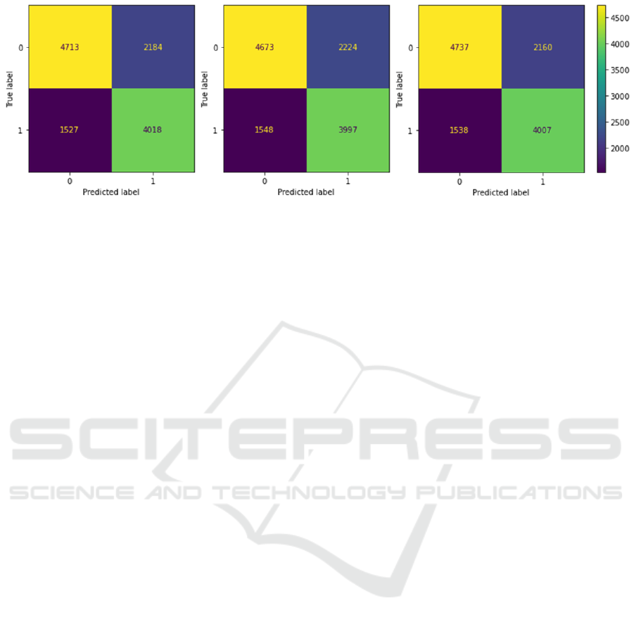
Figure 2: Results obtained with LGB for 3 different feature sets (A, H and W, respectively).

matrices. They show the actual number of TP, TN, FP

and FN cases used for calculating the metric values.

Our evaluation is subject to an external validity

threat (Wohlin et al., 2012) since we conducted a case

study within the context of a single company. Some

of the features in our feature set are also speciﬁc for

the telecommunication domain. More case studies in

different companies and domains must be conducted

to be able to generalize the results.

There are internal validity threats due to the em-

ployed dataset. Although we collected data with tool

support, the data is manually provided by develop-

ers and test engineers. Hence, there might be incor-

rect entries. We preprocessed the collected data to

ﬁx some basic mistakes such as data formatting and

typographical errors. Another issue we noticed was

about the lack of consistency in the use of language

for providing textual descriptions. Some descriptions

were in English, where some others were in Turkish.

We translated Turkish text to English for maintaining

consistency among the descriptions.

The structure of the dataset can lead to construct

validity threats. We employed a variety of metrics to

mitigate these threats. There have been inconsisten-

cies observed regarding the results reported in previ-

ous studies published in the literature, especially be-

tween those that employ open source projects (Bhat-

tacharya and Neamtiu, 2011) and those that employ

commercial projects (Hooimeijer and Weimer, 2007;

Guo et al., 2010) as experimental objects. We sum-

marize related studies in the following section.

5 RELATED WORK

Anbangalan and Wouk (Anbalagan and Vouk, 2009)

reported an empirical study, where the Ubuntu system

was selected as the experimental object. They stud-

ied 72,482 bug reports regarding this system. They

found out that 95% of bug reports are associated with

people of group size ranging between 1 and 8 peo-

ple. They observed a strong linear relationship score

of 92% among the number of users contributing to the

ﬁxing process of a bug and the median time taken to

ﬁx it. They proposed a linear model to predict the

bug ﬁxing time by using the correlation between the

number of people participating in the process and cor-

rection time. We did not consider the number of peo-

ple involved in the bug ﬁxing process as a feature for

classiﬁers. This feature can be considered for very

large scale open source projects like Ubuntu, involv-

ing thousands of contributors. Our dataset does not

involve bug reports regarding a single project. Our

experimental objects include 293 commercial appli-

cations of varying size.

Bhattacharya and Neamtiu (Bhattacharya and

Neamtiu, 2011) constructed regression models for

predicting bug ﬁx time. They employed multivariate

and univariate regression testing. They used a dataset

consisting of 512,474 bug reports. These reports are

collected from Eclipse, Chrome, and three products

of Mozilla. They showed that the accuracy of ex-

isting models ranges between 30% and 49%. They

also found out that bug ﬁx times are not highly corre-

lated with bug-ﬁx likelihood and bug-opener’s repu-

tation. These results contradict with those previously

reported for commercial software projects (Hooimei-

jer and Weimer, 2007; Guo et al., 2010). This shows

that open source projects and commercial projects

might have different properties leading to contradict-

ing results.

Another study (Panjer, 2007) on bug ﬁxing time

prediction utilized Eclipse Bugzilla database, from

which they reached 118,371 bug reports. Instead of

predicting bug ﬁxing time directly, they used a set of

discretized log scaled lifetime classes and they aimed

at predicting the class associated with each bug report.

Hence, they also employed classiﬁers rather than re-

gression models. They experimented with various

prediction models like Na

ıve Bayes, decision trees

On the Use of Machine Learning for Predicting Defect Fix Time Violations

125

and logistic regression. Their feature set includes bug

priority, bug severity, product, component, operating

system, platform, version, target milestone, bug de-

pendencies and comments. However, accuracy of pre-

diction turned out to be very low according to the

reported results. 34,9% is the maximum accuracy,

which was obtained by using logistic regression.

Sawarkar et al. (Sawarkar et al., 2019) achieved

62.52% accuracy in predicting bug ﬁxing time (called

as bug estimation time) with SVM models. They also

predicted the average time that would be required for

each developer. They employed a bag of words model

to predict both the bug ﬁx time and the developer to

be assigned for the task.

Zhang et al. (Zhang et al., 2013) presented an em-

pirical study on predicting bug ﬁxing time for three

projects maintained by CA Technologies. They pro-

posed a Markov-based method to estimate the total

amount of time required to ﬁx a given set of defects.

They also proposed a model to predict the bug ﬁx-

ing time for a particular defect. Hereby, they also ap-

proached the problem as a binary classiﬁcation prob-

lem like we did in our study. They introduced two

classes: slow ﬁx and quick ﬁx. They employed a KNN

classiﬁer to assign a bug report to one of these classes

based on a predetermined time threshold. They mea-

sured an F1 score of 72,45%.

Another study (Ardimento and Dinapoli, 2017)

that tackles the problem as a binary classiﬁcation

problem aims at predicting the resolution time of a

defect as either slow or fast. They performed an em-

pirical investigation for the bugs reported for three

open source projects, namely Novell, OpenOfﬁce and

LiveCode. They used an SVM model as the classiﬁer.

They use features derived from textual descriptions

based on TF-IDF calculations as well. They report ac-

curacy values up to 77%. In our study, we used many

commercial projects as experimental objects and we

experimented with several different types of models

as classiﬁers.

Deep learning models have become very popular

in the recent years and they have also been used for

bug ﬁx time prediction. In particular, BERT (Devlin

et al., 2018) was employed in one of the recent stud-

ies (Ardimento and Mele, 2020). BERT stands for

Bidirectional Encoder Representations from Trans-

formers (Devlin et al., 2018). This model has the abil-

ity to learn the context of word by considering other

words around it in both directions. It was used for

exploiting textual information regarding bug reports

like the comments of developers and bug owners. The

study also adopted a binary classiﬁcation task, where

each bug is assigned to one of the classes called fast

and slow. The median of the number of days it takes

to resolve bugs is selected as the threshold. Resolu-

tions of those bugs of which resolution time (in days)

exceeds this number are categorized as fast. They are

categorized as slow, otherwise. The proposed method

based on the BERT model proved to be very effective,

where the accuracy is measured as 91%. However,

the dataset was obtained from a single open source

project, LiveCode. The size of the dataset is also

small, especially considering the scale of data needed

for a sound assessment of deep learning models.

6 CONCLUSIONS

Fix time of a defect is estimated as soon as a defect

is opened. However, these estimations can turn out

to be inaccurate and as such, the estimated time can

be exceeded. We presented an empirical evaluation on

the use of machine learning for predicting these viola-

tions. We conducted an industrial case study based on

real projects that are being maintained by a telecom-

munications company. We prepared a dataset based

on 69,000 bug reports over the last 6 years regard-

ing 293 projects. We derived 25 features, some of

which are based on textual descriptions. We experi-

mented with 3 different subsets of these features used

for training 7 different classiﬁers. We obtained the

best results with Gradient boosted classiﬁers, which

reached up to 72% accuracy.

REFERENCES

Abhigyan (2020). Understanding logistic regression!!!

https://medium.com/analytics-vidhya/understanding-

logistic-regression-b3c672deac04.

Agrawal, S. (2021). Logistic regression.

https://medium.datadriveninvestor.com/logistic-

regression-1532070cf349.

Anbalagan, P. and Vouk, M. (2009). On predicting the time

taken to correct bug reports in open source projects.

In 2009 IEEE International Conference on Software

Maintenance, pages 523–526. IEEE.

Ardimento, P. and Dinapoli, A. (2017). Knowledge extrac-

tion from on-line open source bug tracking systems

to predict bug-ﬁxing time. In Proceedings of the 7th

International Conference on Web Intelligence, Mining

and Semantics, pages 1–9.

Ardimento, P. and Mele, C. (2020). Using BERT to pre-

dict bug-ﬁxing time. In Proceedings of the IEEE Con-

ference on Evolving and Adaptive Intelligent Systems,

pages 1–7.

Bento, C. (2021). Multilayer perceptron explained with

a real-life example and python code: Sentiment

analysis. https://towardsdatascience.com/multilayer-

ENASE 2022 - 17th International Conference on Evaluation of Novel Approaches to Software Engineering

126

perceptron-explained-with-a-real-life-example-and-

python-code-sentiment-analysis-cb408ee93141.

Bhattacharya, P. and Neamtiu, I. (2011). Bug-ﬁx time pre-

diction models: can we do better? In Proceedings

of the 8th Working Conference on Mining Software

Repositories, pages 207–210.

Bloch, M., Blumberg, S., and Laartz, J. (2012). Deliver-

ing large-scale it projects on time, on budget, and on

value. Harvard Business Review, 5(1):2–7.

Bonaccorso, G. (2017). Machine learning algorithms.

Packt Publishing Ltd.

Choetkiertikul, M., Dam, H. K., Tran, T., and Ghose, A.

(2015). Predicting delays in software projects using

networked classiﬁcation (t). In 2015 30th IEEE/ACM

International Conference on Automated Software En-

gineering (ASE), pages 353–364.

Devlin, J., Chang, M.-W., Lee, K., and Toutanova, K.

(2018). Bert: Pre-training of deep bidirectional trans-

formers for language understanding. arXiv preprint

arXiv:1810.04805.

Ernst, A. M., Lankes, J., Schweda, C. M., and Witten-

burg, A. (2006). Tool support for enterprise architec-

ture management-strengths and weaknesses. In 2006

10th IEEE International Enterprise Distributed Ob-

ject Computing Conference (EDOC’06), pages 13–22.

IEEE.

Guo, P. J., Zimmermann, T., Nagappan, N., and Murphy,

B. (2010). Characterizing and predicting which bugs

get ﬁxed: An empirical study of Microsoft Windows.

In Proceedings of the 32nd ACM/IEEE International

Conference on Software Engineering, page 495–504.

Hao, J. and Ho, T. K. (2019). Machine learning made easy:

a review of scikit-learn package in python program-

ming language. Journal of Educational and Behav-

ioral Statistics, 44(3):348–361.

Hooimeijer, P. and Weimer, W. (2007). Modeling bug re-

port quality. In Proceedings of the 22nd IEEE/ACM

International Conference on Automated Software En-

gineering, page 34–43.

ari

ainen, J. and V

alim

aki, A. (2008). Impact of appli-

cation lifecycle management—a case study. In Enter-

prise Interoperability III, pages 55–67. Springer.

Lee, Y., Lee, S., Lee, C.-G., Yeom, I., and Woo, H.

(2020). Continual prediction of bug-ﬁx time using

deep learning-based activity stream embedding. IEEE

Access, 8:10503–10515.

Magar, B. T., Mali, S., and Abdelfattah, E. (2021). App suc-

cess classiﬁcation using machine learning models. In

2021 IEEE 11th Annual Computing and Communica-

tion Workshop and Conference (CCWC), pages 0642–

0647. IEEE.

Mochalov, V., Bratchenko, N., Linets, G., and Yakovlev,

S. (2019). Distributed management systems for in-

focommunication networks: A model based on TM

forum framework. Computers, 8(2):45.

Morde, V. (2019). Xgboost algorithm: Long may she reign!

https://towardsdatascience.com/https-medium-com-

vishalmorde-xgboost-algorithm-long-she-may-rein-

edd9f99be63d.

Nitin (2020). Lightgbm binary classiﬁcation, multi-

class classiﬁcation, regression using python.

https://nitin9809.medium.com/lightgbm-binary-

classiﬁcation-multi-class-classiﬁcation-regression-

using-python-4f22032b36a2.

Panjer, L. D. (2007). Predicting eclipse bug lifetimes. In

Fourth International Workshop on Mining Software

Repositories (MSR’07: ICSE Workshops 2007), pages

29–29. IEEE.

Parlar, T.,

Ozel, S. A., and Song, F. (2016). Interactions

between term weighting and feature selection meth-

ods on the sentiment analysis of turkish reviews. In

International Conference on Intelligent Text Process-

ing and Computational Linguistics, pages 335–346.

Springer.

Rosenblatt, F. (1958). The perceptron: a probabilistic model

for information storage and organization in the brain.

Psychological review, 65(6):386.

Sawarkar, R., Nagwani, N. K., and Kumar, S. (2019). Pre-

dicting bug estimation time for newly reported bug us-

ing machine learning algorithms. In 2019 IEEE 5th

International Conference for Convergence in Technol-

ogy (I2CT), pages 1–4. IEEE.

Vatsal (2021). K nearest neighbours explained.

https://towardsdatascience.com/k-nearest-

neighbours-explained-7c49853633b6.

Weiss, C., Premraj, R., Zimmermann, T., and Zeller, A.

(2007). How long will it take to ﬁx this bug? In Fourth

International Workshop on Mining Software Reposito-

ries (MSR’07:ICSE Workshops 2007), pages 1–1.

Wohlin, C., Runeson, P., Host, M., Ohlsson, M., Regnell,

B., and Wesslen, A. (2012). Experimentation in Soft-

ware Engineering. Springer-Verlag, Berlin, Heidel-

berg.

Yadav, A. (2018). Support vector machines(svm).

https://towardsdatascience.com/support-vector-

machines-svm-c9ef22815589.

Yiu, T. (2021). Understanding random forest.

https://towardsdatascience.com/understanding-

random-forest-58381e0602d2.

Zhang, H., Gong, L., and Versteeg, S. (2013). Predicting

bug-ﬁxing time: an empirical study of commercial

software projects. In Proceedings of the 35th Inter-

national Conference on Software Engineering, pages

1042–1051.

On the Use of Machine Learning for Predicting Defect Fix Time Violations

127