An Image Quality Assessment Method

based on Sparse Neighbor Signiﬁcance

Selcuk Ilhan Aydi

Institute of Science, Faculty of Computer Engineering, Gebze Technical University, Turkey

Keywords:

Image Quality Assessment, Sparse Coding, Human Visual System.

Abstract:

In this paper, the image quality assessment problem is tackled from a sparse coding perspective, and a new

automated image quality assessment algorithm is presented. Speciﬁcally, the input image is ﬁrst divided into

non-overlapping blocks and sparse coding is used to reconstruct a central sub-block using the neighboring

sub-blocks as dictionaries. The resulting 2D sparse vectors from each neighboring sub-block, are devised

as signiﬁcance maps that are then used in similarity measures between the reference and distorted images.

The proposed method is compared against various recently introduced shallow and deep methods across four

datasets and multiple distortion types. The experimental results that have been obtained show that it possesses

a strong correlation with the Human Visual System and outperforms its counterparts.

1 INTRODUCTION

Image quality assessment (IQA) is a difﬁcult task due

to the not yet fully understood Human Visual System

(HVS). The HVS has a complex behavior during the

process of rating the quality of visual content. Over

the past few decades, many objective image quality

assessment methods have been developed. IQA mod-

els may be categorized as full-reference (FR-IQA),

reduced-reference (RR-IQA), and no-reference (NR-

IQA). In the case of FR-IQA, the reference version of

the distorted image is available, while only partial in-

formation is provided in the second category. In the

case of NR-IQA, the reference image is unavailable.

The present study focuses on the ﬁrst case.

Two main IQA strategies have met with wide ac-

claim by the scientiﬁc community (Wang and Bovik,

2006). The ﬁrst is the error sensitivity paradigm,

where an error signal is obtained, which is assumed

to be a quality measurement. The primitive methods

using error sensitivity, including mean squared error

(MSE), peak signal-to-noise ratio (PSNR), do not cor-

relate well with the HVS (Wang and Bovik, 2006).

Another difﬁculty concerns distinguishing distortion

types with the same error value. The second ap-

proach, known as structural similarity index (SSIM)

(Zhou Wang et al., 2004), is based on the assumption

that the HVS focuses on structural information (Wang

et al., 2002). It is motivated by the internal mecha-

nism of the HVS, where hierarchical pre-processing

is known to be conducted in order to extract progres-

sively more complex object-level information (Wang

and Bovik, 2006).

In both approaches, the main challenge consists

of dealing with the different types of distortions that

may lead to various divergent or convergent results

in terms of quality scores (Wang and Bovik, 2006).

In this paper, an IQA method based on sparse cod-

ing called Sparse Signiﬁcance Image Quality Mea-

sure (SSIQM) has been developed, that deals explic-

itly with structural distortion types.

Recently, sparse coding has been a promising ap-

proach in the domain of image quality assessment

(Guha et al., 2014; Li et al., 2016; Liu et al., 2017). It

also has a strong consistency with the HVS.

The perception of the scene by the HVS has the

following procedures. The continuous stream of vi-

sual stimuli projected on retina is transmitted to the

primary visual cortex (V1) through the Lateral Genic-

ulate Nucleus (LGN) for the abstraction process. The

extensive experiments show that the underlying pro-

cess of the brain is heavily based on reducing the re-

dundancy presents in the visual stimuli and not only

the visual cortex but also the other parts of the brain

are involved in this process. If it is assumed that for

each image the weights of each neuron is different

then utilizing the weights of each neuron in the IQA

is feasible to implement an IQA method. Such a be-

havior of the HVS can be well modelled using sparse

coding, in the sense of atoms in the dictionary have

different weights and corresponds to different signiﬁ-

cance.

Speciﬁcally sparse coding represents a signal via

a linear combination using a set of basis functions

Aydi, S.

An Image Quality Assessment Method based on Sparse Neighbor Signiﬁcance.

DOI: 10.5220/0011058700003209

In Proceedings of the 2nd International Conference on Image Processing and Vision Engineering (IMPROVE 2022), pages 34-44

ISBN: 978-989-758-563-0; ISSN: 2795-4943

and their corresponding coefﬁcients and is widely ac-

cepted as a process related to the cognitive behavior

of the HVS (Olshausen and Field, 1996; Olshausen

and Field, 1997; Comon, 1994; Bell and Sejnowski,

1995; Lee et al., 1999; A. Hyv

arinen and E. Oja,

2010). Sparse Feature Fidelity (Chang et al., 2013)

and Adaptive Sub-Dictionary Selection Strategy (Li

et al., 2016) learn dictionaries to represent any dis-

torted image in linear relation with sparse vector and

employ this sparse coefﬁcients in the calculation of

objective quality of the distorted image.

In addition to the idea of using sparse coding in

IQA, the neighboring blocks are also considered in

the design of SSIQM. From the perspective of biol-

ogy, a phenomenon known as visual agnosia (Farah,

2004), refers to the impairment of the visual stimuli in

the process of recognition of objects. In general, there

exist two types of agnosia, including apperceptive ag-

nosia and associative agnosia. In the former, patients

can recognize the local features of the visual informa-

tion projected on the retina. However, patients cannot

correctly perceive the adjacent features that are con-

tributing to the actual structure of the visual object.

As a result, considering the neighboring blocks in the

IQA problem is crucial and consistent with the visual

perception of the HVS.

Furthermore, many pieces of research support the

fact that the use of neighboring blocks is an important

approach in visual recognition (Khellah, 2011; Qian

et al., 2013). In (Khellah, 2011), the author employ-

ees a pixel-based similarity map, is constructed by

utilizing the dominant neighborhood structure for tex-

ture classiﬁcation. In (Qian et al., 2013), the authors

aim to use a relationship between the center pixel and

its neighboring pixels, is deﬁned by linear representa-

tion coefﬁcients determined using ridge regression in

the problem of face recognition.

In this paper, an IQA method based on sparse cod-

ing called Sparse Signiﬁcance Image Quality Mea-

sure (SSIQM) has been developed, that deals explic-

itly with structural distortion types. SSIQM takes into

account the relationship of the neighboring blocks in

terms of sparse signiﬁcance.

This article’s contributions can be summarized as

follows:

1. A novel FR-IQA method, adopting sparse feature

vectors is proposed; the sparse vectors are ex-

tracted via dynamic dictionaries constructed from

normalized pixel intensities of image patches

(neighboring blocks of the center block), instead

of using ﬁxed over-complete orthogonal dictio-

naries. Moreover, gradient information, known

to be well-correlated (Xue et al., 2014) with the

HVS is also exploited. Also, on the contrary of

alternative approaches, the proposed SSIQM does

not require input image sanitation as preprocess-

ing.

2. This approach assumes that the neighboring

blocks may affect the perceptual quality of the

center block and this implicit relation between the

neighboring and center blocks may be reveled by

sparse coding. Hence, the sparse signiﬁcance re-

lation between the center block and its neighbors

are investigated. Instead of comparing the ref-

erence and distorted images directly, a similarity

metric is developed processing on sparse signif-

icance maps. These maps are constructed in a

novel manner; the center block is used as the sig-

nal of interest and the neighbour blocks are uti-

lized as dictionaries. The sparse feature vectors

are then considered as the feature sets to be used

in the quality assessment.

In the remainder of this article, ﬁrst an overview of

related studies (Section 2), including sparse based

methods, are provided. Next, in Section 3 the details

of the proposed method are presented. Then, in Sec-

tion 4 the results of an extensive set of experiments

are discussed. The article concludes with Section 5

where future directions of research are provided.

2 RELATED WORKS

The approaches addressing the FR-IQA problem,

can be divided into three main categories: error-

sensitivity, structural similarity and information the-

oretic (Wang and Bovik, 2006).

2.1 Error Sensitivity based Methods

The methods under this category measure the errors

between reference and distorted images via known

features of the HVS. There are several methods based

on the concept of error sensitivity, e.g. Perceptual Im-

age Distortion (PID) (Teo and Heeger, 1994), Noise

Quality Index (NQM) (Damera-Venkata et al., 2000)

and, Visual Signal-to-Noise Ratio (VSNR) (Chandler

and Hemami, 2007), operating on the contrast sen-

sitivity function, luminance adaptation, and contrast

masking features of the HVS to deal with the IQA

problem.

Most Apparent Distortion (MAD) (Larson and

Chandler, 2010) assumes that the HVS has a different

sensitivity to the different degrees of distortion in im-

ages. The basic assumption is that the HVS tends to

be sensitive to the distortions in relatively more qual-

ity images, whereas the HVS looks for image content

An Image Quality Assessment Method based on Sparse Neighbor Signiﬁcance

in low-quality images. By following this hypothesis,

MAD proposes two models simulating the underlying

mechanism of the HVS and ﬁnally provides a distor-

tion measure.

The Visible Differences Predictor (VDP) (Daly,

1992) looks for the probability of difference between

two images. VDP produces a probability-of-detection

map between the reference and distorted image. The

map is utilized in the subsequent stages to obtain a

ﬁnal quality score.

Watson’s DCT model (Watson, 1993) is based on

DCT coefﬁcients of local blocks. It ﬁrst divides the

image into DCT sub-blocks and calculates a visibility

threshold for each coefﬁcient in each sub-block. The

DC coefﬁcients of DCT blocks are then normalized

by the average luminance. The model also addresses

the contrast/texture masking determined by all the co-

efﬁcients within the same block. In the next stage, the

errors are normalized between the reference and dis-

torted image. At the ﬁnal phase, the errors and fre-

quencies are pooled together, and a ﬁnal quality score

is obtained.

2.2 Structural Information based

Methods

As far as structural information is concerned, the

milestone method might be the Structural Similarity

Index (SSIM) that incorporates luminance, contrast,

and structural information as a feature set to evaluate

the distorted image’s quality perceived by the HVS.

Many extensions to SSIM have been proposed, such

as Multiscale SSIM (M-SSIM) (Wang et al., 2003)

and Information content weighted SSIM (IW-SSIM)

(Wang and Li, 2011).

The Gradient Similarity-based FR-IQA method

(GSM) (Zhu and Wang, 2011) uses four directional

high-pass ﬁlters to calculate the variations in con-

trast/structural information in images. Another exam-

ple in this category, considering the fact that the HVS

tends to be sensitive to low level features at key lo-

cations such as edges (Stevens, 2012), the Riesz Fea-

ture Similarity index (Zhang et al., 2010) employs the

Riesz transform to characterize local structures in an

image at edges formed by Canny operator. In addition

to that, the frequency domain is essential in quality

assessment algorithms. A representative method that

deals with frequency is the Feature Similarity index

(FSIM) (Zhang et al., 2011), which uses phase con-

gruency and gradient magnitude as complementary

features to detect visual quality in images. Phase con-

gruency is utilized as a weighting function to provide

single similarity for each sub-block, supporting the

fact that the phase information is more important than

the gradient magnitude. Another method that uses

phase and gradient components is the Visual Saliency

Index (VSI) (Zhang et al., 2014). Phase information

is used to calculate visual saliency with some priors

and, the gradient magnitude is obtained by the Scharr

gradient operator.

In addition to these methods, gradient variation in-

formation has been an important feature to be consid-

ered in the quality problem (Liu et al., 2011). Gra-

dient Magnitude Similarity Deviation (GMSD) (Xue

et al., 2014) assumes that gradients have a more

meaningful variation to image distortions and, this

behavior may point out the quality of an image per-

ceived by the HVS.

Structural Contrast Quality Index (SC-IQ) (Bae

and Kim, 2016) has been recently proposed and, it

deals well with various structural distortion types and

has been developed on top of the Structural Contrast

Index (SCI) (Bae and Kim, 2014). SCI can detect per-

ceived distortion for many different distortion types.

It deﬁnes the structural distortion as the ratio of struc-

tureness and contrast intensity, where the structure-

ness is deﬁned as the kurtosis of the magnitudes of

DCT AC coefﬁcients, and contrast intensity is deﬁned

as the ratio of mean and square of N, where N is the

height (= width) of NxN DCT block. By following

this index, SC-IQ employs SCI as a feature in the de-

sign of IQA method. In addition to that, SC-IQ de-

vises chrominance values to reﬂect the effect of the

color components on perceived quality (Zhang et al.,

2011) (Zhang et al., 2014). Moreover, to reﬂect the

contrast sensitivity function (CSF) of the HVS, SC-

IQ introduces three frequency domain measures by

comparing contrast energy values in high frequency,

middle frequency and low frequency.

2.3 Information Theoretic based

Methods

From the perspective of this category, image qual-

ity assessment is treated as an information ﬁdelity

problem. The basic idea is to model a communica-

tion channel between the image distortion process and

the visual perception process. This approach seeks

the answer to the question: how much information is

shared between the reference and distorted image?

A representative and successful implementation

in this category, Visual Information Fidelity (VIF)

(Sheikh and Bovik, 2006), quantiﬁes the perceived

information present in the reference image and the

amount of this reference information extracted from

the distorted image. These two measures are com-

bined, and the VIF index is proposed as the model

output. This model is an extension of its former

IMPROVE 2022 - 2nd International Conference on Image Processing and Vision Engineering

method Information Fidelity Criterion (IFC) (Sheikh

et al., 2005).

2.4 Sparse Coding based Approaches

In the ﬁeld of image quality assessment, many effec-

tive approaches attempt to mimic the HVS. Some of

them use structural information and integrate this in-

formation with sparse coding techniques to give some

meaningful weights to extracted structural features

and blocks. However, sparse coding-based methods

generally waste time in the training stage to learn dic-

tionaries from the reference image set. Moreover,

training on the dictionary is very speciﬁc to the used

dataset. In this section, a review of such methods is

presented.

In the ﬁrst method, Sparse Feature Fidelity

(Chang et al., 2013), the weighting matrix is learned

by machine learning and, the resulting matrix is used

to ﬁnd the sparsest feature map by using Independent

Component Analysis (ICA). The calculated sparse

features are utilized as a feature set to be used in qual-

ity assessment. Sparse Feature Fidelity (SFF) also

combines luminance correlation with sparse feature

to enhance the correlation with the HVS.

In the second method, Adaptive Sub-Dictionary

Selection Strategy (Li et al., 2016) ﬁrstly, an over-

complete visual dictionary which is used to represent

the reference image in the feature extraction phase, is

learned by utilizing a set of natural images. The dis-

torted image is represented by the sub-dictionary that

is obtained from the over-complete dictionary used

in the representation of the reference image. More-

over on this, to enhance the performance of the pro-

posed method, a number of auxiliary features includ-

ing, contrast, color and luminance are employed to be

able to reﬂect the HVS behavior more precisely.

The third method, Kernel Sparse Coding Based

Metric (Zhou et al., 2021) approaches the IQA from

a nonlinear perspective to better reveal the structures

which provide an effective representation of image

patches. In addition to that, sparse coding coefﬁcients

and reconstruction error are utilized to construct a ﬁ-

nal quality score. However, this approach has many

parameters and computationally inefﬁcient.

In the fourth method, Sparseness Signiﬁcance

Ranking Measure (Ahar et al., 2018), the general idea

is to rank Fourier components by their signiﬁcance to

provide a quality metric. The Fourier basis are used as

complete-dictionaries for sparse coding and a ranking

mechanism is provided. A sparse analysis of AC and

DC components is performed and pooled to calculate

a ﬁnal quality score.

3 PROPOSED METHOD

3.1 Sparse Coding

Sparse coding represents a given signal in a linear

combination of two components: the ﬁrst is a dic-

tionary or weight vector, the latter is the sparse fea-

ture vector (Wang et al., 2015). In other words, the

main goal is to ﬁnd a set of basis functions having

linear combinations with sparse features. Generally

speaking, a sparse feature vector/matrix has mostly

zero components, pointing out its sparsity. A given

signal, x, present in a high dimensional space R

, can

be represented using D ∈ R

m×n

, with n atoms as

x = Ds (1)

where D is a dictionary of atoms extracted or learned

and s is a sparse feature vector. The sparsest vector

s can be found by solving the following optimization

problem

min

kDs − xk

+ λksk

(2)

where λ is an adjustment parameter to balance be-

tween reconstruction error and sparsity. The l

-norm

denoted by k.k

, counts the number of zero elements

in sparse vector. If D is properly chosen then, s tends

to have values of zero or close to zero.

3.2 SSIQM

SSIQM consists of two pipelines executing in par-

allel to each other. The ﬁrst pipeline constructs the

sparse signiﬁcance maps while the second pipeline

deals with gradient information extraction for each

sub-block. The outputs of the underlying pipelines

are pooled at the ﬁnal phase, producing quality score.

Preprocessing stage converts the RGB color space to

grayscale and a unity-based min-max normalization

is employed to rescale the intensity values to scale the

range in [0, 1]. In addition to that, the input images are

down-scaled to a ﬁxed size of 128×128 by perform-

ing interpolation for the sake of computational com-

plexity. The experimental results show that directly

converting from RGB to grayscale produces more ef-

ﬁcient results. To sum up, SSIQM can be shown as

SSIQM = F(I

,β,γ,θ) (3)

where β and γ are the weights of sparse signiﬁcance

map and gradient similarity scores, respectively, θ

points to internal parameters including window size

and sparse coding parameters. I

and I

denote

the reference and distorted images, respectively. An

overview of SSIQM is illustrated in Fig.1.

In the ﬁrst pipeline, the input image is divided into

15×15 blocks and then each block is divided into ﬁve

An Image Quality Assessment Method based on Sparse Neighbor Signiﬁcance

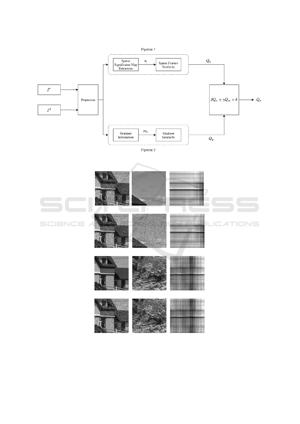
Figure 1: General SSIQM design, having two parallel pipelines calculating gradient and sparse signiﬁcance maps. The global

quality scores produced by pipelines are pooled in the last step, offering an objective quality score.

(a) (b) (c)

(d) (e) (f)

(g) (h) (i)

(j) (k) (l)

Figure 2: Reference and distorted local blocks, and their corresponding north, south and signiﬁcance maps. a and d are the

same reference center local blocks, g and j are the the same distorted center local blocks, b and e are the north local blocks

of the reference and distorted local blocks, h and k are the north and south local blocks of the reference and distorted local

blocks. The latest column c, f, i and l are the sparse signiﬁcance maps of the pair of center and its neighbour local blocks.

IMPROVE 2022 - 2nd International Conference on Image Processing and Vision Engineering

sub-blocks. Each sub-block consists of the center c

i∈{1,...,M} and its 4-neighbors n

i, j

, j∈{1, 2, 3, 4}.

Each n

i, j

block is used as D in (2). The center block

is used as the signal of interest, x, in (2) and, a sparse

coding algorithm A(c,n) is utilized to obtain sparse

vectors. For each center block, c

, four sparse signif-

icance maps are constructed using the sparse vectors,

, resulting a set of pairs of (n

i, j

). Final sparse

signiﬁcance maps are then, forwarded to a local sim-

ilarity function, providing the local quality for each

pair. In this study, a well-known structural similarity

measure is adapted as the local quality function

q(x

) =

+ δ

+ 2y

+ δ

(4)

where x

and y

are the two image patches and δ

used to avoid zero division. The resulting normalized

global similarity Q

between the reference and dis-

torted signiﬁcance maps can be derived from equation

4 as

= 1/M

∑

i=1

+ δ

+ S

+ δ

(5)

where S

and S

are the signiﬁcance maps of the

i − th center block extracted from the reference and

distorted images, respectively. This ﬁnal normal-

ized score represents the global similarity in terms of

sparse signiﬁcance.

The reason of using direct pixel values is in order

to ﬁnd a relationship in the pixel domain in terms of

sparse signiﬁcance. Since SSIQM does not prioritize

representing a signal in a lower dimensional space,

the neighbouring local blocks are used as complete

dictionaries. On the other hand, a frequency level

dictionary might also be used such as, DCT or FFT

components. In this situation, a relationship may be

captured in the frequency domain, which is however

out of the scope of this work.

A number of sparse signiﬁcance maps and the cor-

responding dictionaries with the center local blocks

are illustrated in Fig.2. The sparse signiﬁcance maps

are shown in the last column for each pair of center

and its neighbour block. The distortion type used in

Fig.2 is additive gaussian noise. Whiter pixels in the

signiﬁcance maps represent a strong weight whereas

darker pixels exhibit weak weight for each atom in the

dictionary.

In Fig.2, each column in the signiﬁcance maps

represent a weight vector for each column in the dic-

tionaries/neighbour blocks. It can be observed that

the signiﬁcance maps have a correlation with the sim-

ilarity between the center and neighbour blocks. In

other words, the sparse coding algorithm uses almost

all the atoms in the dictionary to be able to recon-

struct the original image when the pixel-level similar-

ity between the center and neighbour block is lower.

Noticeably, the signiﬁcance maps are sensitive to the

distortions as it is depicted in Fig.2(c), 2(f) and 2(i),

2(l), where the variations in the maps are quite visible.

There are many sparse coding algorithms imple-

mented and ready to use in literature. In this paper,

threshold is selected as sparse coding algorithm de-

noted by A(c,n), implemented in (Pedregosa et al.,

2011) that squashes to zero all coefﬁcients of sparse

vector less than the given threshold.

In the second pipeline, the magnitude information

is extracted from the reference and distorted images.

We used the Robert’s cross edge detector to ﬁnd the

edges which correlates to the HVS relatively better

compared to the Sobel ﬁlter according to our experi-

ments. The magnitude P can be shown as

P =

+ g

(6)

where g

and g

are the direction in both axis. The

normalized magnitude map m produced by equation

6, is then divided into 15×15 blocks. The magnitude

similarity, Q

, for each block extracted from the ref-

erence and distorted image is then calculated as

= 1/M

∑

i=1

+ δ

+ m

+ δ

(7)

where m

and m

are i − th local block magnitude

maps of the reference and distorted images, respec-

tively.

In the latest stage, Q

and Q

are pooled to pro-

vide a ﬁnal objective quality score Q

for the given

distorted image. Both quality scores have their own

weights in the pooling stage as

= βQ

+ γQ

+ b (8)

In equation 8, b is used to avoid zero quality score.

Instead of determining β, γ and b by ad-hoc methods,

Support Vector Regression (SVM) is used to obtain

more effective results.

4 EXPERIMENTAL RESULTS

This section presents the performance analysis and re-

sults gathered from different experiments conducted

on well-known subjective datasets; TID2008 (Pono-

marenko et al., 2009), TID2013 (Ponomarenko et al.,

2015), CSIQ (Larson and Chandler, 2010) and LIVE

(Sheikh et al., 2006), and a set of comparisons are

demonstrated with a number of state-of-the-art IQMs.

TID2008 has 1700 distorted images, 25 reference

images, having 17 distortion types with 4 levels.

An Image Quality Assessment Method based on Sparse Neighbor Signiﬁcance

Table 1: Comparison of SSIQM vs. seven state of the art IQMs on four datasets with ﬁve performance metrics.

Method Criteria

TID2013 TID2018 LIVE CSIQ

PSNR

SRCC 0.754 0.672 0.819 0.887

PRCC 0.732 0.641 0.800 0.897

KRCC 0.548 0.453 0.617 0.685

RMSE 22.90 21.65 28.19 29.94

SSIM (Zhou Wang et al., 2004)

SRCC 0.728 0.694 0.874 0.890

PRCC 0.735 0.679 0.713 0.807

KRCC 0.535 0.500 0.687 0.695

RMSE 3.700 3.687 0.291 0.322

MS-SSIM (Wang et al., 2003)

SRCC 0.799 0.769 0.877 0.918

PRCC 0.770 0.734 0.665 0.826

KRCC 0.597 0.567 0.687 0.742

RMSE 3.659 3.634 0.334 0.336

VIFp (Sheikh and Bovik, 2006)

SRCC 0.538 0.594 0.869 0.886

PRCC 0.538 0.523 0.858 0.890

KRCC 0.432 0.439 0.677 0.790

RMSE 4.032 4.040 0.187 0.163

FSIMc (Zhang et al., 2011)

SRCC 0.869 0.902 0.919 0.899

PRCC 0.849 0.845 0.776 0.827

KRCC 0.686 0.718 0.748 0.709

RMSE 3.644 3.609 0.356 0.356

GMSD (Xue et al., 2014)

SRCC 0.810 0.896 0.909 0.947

PRCC 0.859 0.868 0.866 0.938

KRCC 0.644 0.714 0.730 0.796

RMSE 4.502 4.430 0.510 0.095

UQI (Zhou Wang and Bovik, 2002)

SRCC 0.707 0.567 0.786 0.589

PRCC 0.530 0.418 0.450 0.419

KRCC 0.505 0.393 0.579 0.420

RMSE 3.616 3.576 0.441 0.354

SSIQM proposed

SRCC 0.883 0.890 0.914 0.937

PRCC 0.790 0.794 0.679 0.855

KRCC 0.702 0.711 0.728 0.772

RMSE 7.770 7.709 11.05 11.22

Table 2: Comparison of SSIQM vs. ten state of the art FR/NR CNN Based IQMs on three datasets with two performance

metrics.

Method Criteria

TID2013 LIVE CSIQ

H-IQA (Lin and Wang, 2018)

SRCC 0.790 0.982 0.885

PRCC 0.880 0.982 0.910

AIGQA (Ma et al., 2021)

SRCC 0.871 0.960 0.885

PRCC 0.893 0.957 0.952

BPSQM (Pan et al., 2018)

SRCC 0.862 0.973 0.927

PRCC 0.885 0.963 0.952

DB-CNN (Zhang et al., 2018)

SRCC 0.816 0.968 0.874

PRCC 0.865 0.971 0.915

BIECON (Kim and Lee,

2016)

SRCC 0.717 0.958 0.946

PRCC 0.762 0.960 0.959

DIQA (Kim et al., 2018)

SRCC 0.825 0.975 0.884

PRCC 0.850 0.977 0.915

CaHDC (Wu et al., 2020)

SRCC 0.862 0.965 0.903

PRCC 0.878 0.964 0.914

DSIR-IQA (Liang et al.,

2021)

SRCC 0.782 0.967 0.820

PRCC 0.816 0.969 0.878

DMIR-IQA (Liang et al.,

2021)

SRCC 0.796 0.967 0.823

PRCC 0.821 0.971 0.881

SSIQM proposed

SRCC 0.883 0.914 0.937

PRCC 0.790 0.679 0.855

IMPROVE 2022 - 2nd International Conference on Image Processing and Vision Engineering

Table 3: Comparison of SRCC of CNN Based Models and SSIQM in cross dataset test.

Trained Tested

AIGQA

(Ma et al., 2021)

DIQA

(Kim et al., 2018)

DSIR-IQA

(Liang et al., 2021)

DMIR-IQA

(Liang et al., 2021)

SSIQM

proposed

TID2013

LIVE 0.886 0.904 0.879 0.880 0.914

CSIQ 0.823 0.877 0.856 0.867 0.937

LIVE

TID2013 0.698 0.922 0.878 0.891 0.883

CSIQ 0.847 0.915 0.903 0.922 0.937

CSIQ

LIVE - 0.926 0.936 0.947 0.914

TID2013 - 0.923 0.906 0.907 0.883

Table 4: Performance of SSIQM on individual distortions of TID2013.

Type SRCC PRCC KRCC RMSE

Additive Gaussian noise 0.938 0.850 0.759 7.693

Noise in color components 0.876 0.866 0.683 7.260

Spatially correl. Noise 0.920 0.857 0.737 7.697

Masked noise 0.827 0.747 0.632 7.310

High frequency noise 0.928 0.878 0.748 7.626

Impulse noise 0.885 0.795 0.700 8.361

Quantization noise 0.906 0.773 0.721 7.536

Gaussian blur 0.974 0.876 0.862 7.878

Image denoising 0.963 0.890 0.840 7.431

JPEG compression 0.948 0.918 0.793 7.762

JPEG2000 compression 0.960 0.887 0.832 8.023

JPEG transm. Errors 0.887 0.822 0.656 7.67

JPEG2000 transm. Errors 0.889 0.779 0.701 8.005

Non ecc. patt. Noise 0.785 0.701 0.535 7.130

Local block-wise dist 0.613 0.561 0.433 8.687

Mean shift 0.592 0.539 0.409 3.690

Contrast change 0.429 0.575 0.297 5.997

Change of color saturation 0.478 0.305 0.329 8.334

Multipl. Gauss. Noise 0.911 0.842 0.727 7.787

Comfort noise 0.924 0.861 0.755 7.471

Lossy compr. of noisy images 0.941 0.868 0.783 7.742

Image color quant. w. dither 0.921 0.809 0.748 7.672

Chromatic aberrations 0.884 0.826 0.720 7.365

Sparse sampl. and reconstr 0.966 0.874 0.836 7.890

TID2013 dataset has 3000 distorted images, 25 ref-

erence images, and 24 distortion types with 5 levels.

CSIQ has 866 distorted images, 30 reference images

with 6 distortion types in 5 levels. On the other hand,

the LIVE dataset has 779 distorted images based on

29 references that are subjected to 5 different distor-

tion types at different distortion levels.

The experiments conducted in this section consist

of two categories: comparing SSIQM with statisti-

cal and CNN-based methods. In addition, the perfor-

mance of SSIQM on different distortion types is stud-

ied. It is assumed that an ideal IQA method should en-

sure a correlation with the HVS without any internal

layer between objective and subjective scores. That

is why, any logistic regression method between ob-

jective and subjective scores has not been performed

in this study. Since this paper focuses on structural

degradation, contrast and mean shift distortion types

are excluded from all experiments.

In the ﬁrst experiment, PSNR, SSIM (Zhou Wang

et al., 2004), MS-SSIM (Wang et al., 2003), VIF

(Sheikh and Bovik, 2006), FSIMc (Zhang et al.,

2011), GMSD (Xue et al., 2013) and UQI (Zhou

Wang and Bovik, 2002) are compared to the pro-

posed method SSIQM in terms of correlation with

the HVS. All these methods are implemented and

performed with their default values. To be able to

evaluate the performance of each IQMs four metrics

are employed, including Pearson’s linear correlation

coefﬁcient (PLCC), Spearman rank-order correlation

coefﬁcient, Kendall rank-order correlation coefﬁcient

(KRCC), and root mean squared error (RMSE).

The overall performance of SSIQM is shown in

Table 1 with seven alternative methods and four met-

An Image Quality Assessment Method based on Sparse Neighbor Signiﬁcance

rics on four datasets. The most successful results are

highlighted in bold. From Table 1, on TID2013, it can

be observed that SSIQM has superior performance

over the other full reference IQA methods speciﬁcally

in terms of prediction accuracy while FSIMc shows

a better monotonic performance than SSIQM in this

dataset. Moreover, RMSE is higher than SSIQM and

PSNR. This is mainly due to the fact that SSIQM

does not have an optimized pooling strategy. On

the TID2008 dataset, although GMSD and FSIMc

have a higher correlation, SSIQM presents a com-

petitive performance in terms of prediction accuracy.

On the other hand, SSIQM has a worse PRCC score.

The proposed method has competitive performance

against SSIM, MS-SSIM, FSIMc, and GMSD on the

LIVE dataset. On CSIQ, SSIQM is not at the ﬁrst

rank, however, it exhibits a competitive prediction ac-

curacy and a fair level of PRCC.

When deep models are trained on one dataset they

can produce good results if the test dataset is the same

as the training set that has the same distortion types.

Moreover, cross dataset tests show the real generaliza-

tion of deep models where they are trained on dataset

X and evaluated on dataset Y. However, the general

challenging problem is the lack of dataset to be used at

the training phase which leads to over-ﬁtting in most

of the cases if the number of parameters of the deep

model is relatively big enough. To tackle down this

problem, most of the papers use augmentation tech-

niques to increase the number of items in a dataset

that will help avoid the over-ﬁtting problem. This

may provide some performance improvement but lo-

cal qualities and their importance are not distributed

uniformly in most of the distortion types.

In the second experiment of setup, SSIQM is com-

pared against CNN based methods including, H-IQA

(Lin and Wang, 2018), AIGOA (Ma et al., 2021),

BPSQM (Pan et al., 2018), DB-CNN (Zhang et al.,

2018), BIECON (Kim and Lee, 2016), DIQA (Kim

et al., 2018), CaHDC (Wu et al., 2020), DSIR-IQA

and DMIR-IQA (Liang et al., 2021). The overall per-

formance of each deep model is illustrated in Table 2,

showing only SRCC and PRCC scores and compar-

ing them with SSIQM. All the models are trained and

validated in the same dataset in each row. It is pos-

sible to notice that SSIQM has a superior prediction

accuracy on TID2013 while its SRCC is competitive

to others. On LIVE and CSIQ, deep models generally

have higher performance whereas SSIQM performs

well and its accuracy is promising.

Furthermore, the cross dataset test is conducted to

measure the power of SSIQM on LIVE, CSIQ, and

TID2013 databases. For this experiment the com-

mon distortion types among the three databases are

selected including, GB, WN, JPEG, and JPEG200

and the methods used including, AIGQA, DIQA,

DSIR-IQA, and DMIR-IQA. Table 3 demonstrates

the SRCC results of cross dataset test. It can be ob-

served that SSIQM performs best when deep models

are trained on TID2013 and tested with other datasets.

DIQA has a better generalization capability compared

to other deep models. Training on LIVE and vali-

dating on other datasets gives better scores for DIQA

while other models follow a stable graph. On the

other hand, SSIQM’s performance is the best in the

CSIQ dataset compared to others. When the training

dataset is CSIQ, deep models have higher prediction

accuracy than SSIQM.

Each distortion type has its own effect on differ-

ent aspects of an image that potentially may alter the

perception of the scene by the HVS. To determine the

performance of SSIQM on variety of distortions an

experiment is conducted and the results are shown in

Table 4. It can be seen that, SSIQM has a strong cor-

relation in a wide range of distortion set in TID2013.

It performs best in structural and non-color distortions

while its performance is not sufﬁcient in mean shift,

contrast change, change of color saturation and local

block-wise distortion and the corresponding rows are

in bold. Since SSIQM only relies on two extracted

features it does not address all kinds of degradation,

however, the performance on failed distortions might

be enhanced by adding new features which are im-

portant for the perception of the HVS. The underly-

ing features might be sensitive to color components,

contrast information, and light adaptation.

5 CONCLUSION

In conclusion, it can be established that the pro-

posed method works well with most of the distortion

types except mean shift and contrast. To be able to

determine the performance of the proposed method

we conducted intensive experiments where SSIQM is

ﬁrst compared with the most successful statistical FR-

IQA methods. Furthermore, SSIQM’s performance is

compared with deep models on different datasets via

cross dataset tests. Since each distortion has different

effects on perceptual quality SSIQM’s performance

on each distortion type has been measured. From

the experiments we can conclude that our proposed

method has a good correlation with HVS on many

distortion types. Its performance is very competitive

with a simple design when its counterparts are con-

sidered.

A further study would be adding more features

considering the aspects of HVS to provide a more

IMPROVE 2022 - 2nd International Conference on Image Processing and Vision Engineering

robust IQA method on all the distortion types and

databases. It is also possible to integrate the sparse

signiﬁcance maps with the modern deep models. Fi-

nally, we would like to remark that SSIQM shows a

well moderate correlation with the HVS and holding

the promise to evaluate the images in a robust and ef-

fective manner when it is used in video codecs and

applications that consider image quality.

REFERENCES

A. Hyv

arinen, J. K. and E. Oja, J. W. (2010). Independent

component analysis. New York, NY, 62(3):412–416.

Ahar, A., Barri, A., and Schelkens, P. (2018). From sparse

coding signiﬁcance to perceptual quality: A new ap-

proach for image quality assessment. IEEE Transac-

tions on Image Processing, 27(2):879–893.

Bae, S.-H. and Kim, M. (2014). A novel generalized dct-

based jnd proﬁle based on an elaborate cm-jnd model

for variable block-sized transforms in monochrome

images. IEEE Transactions on Image Processing,

23(8):3227–3240.

Bae, S.-H. and Kim, M. (2016). A novel image quality as-

sessment with globally and locally consilient visual

quality perception. IEEE Transactions on Image Pro-

cessing, 25(5):2392–2406.

Bell, A. J. and Sejnowski, T. J. (1995). An information-

maximization approach to blind separation and blind

deconvolution. Neural computation, 7(6):1129–1159.

Chandler, D. M. and Hemami, S. S. (2007). Vsnr: A

wavelet-based visual signal-to-noise ratio for natural

images. IEEE Transactions on Image Processing,

16(9):2284–2298.

Chang, H.-W., Yang, H., Gan, Y., and Wang, M.-H. (2013).

Sparse feature ﬁdelity for perceptual image quality as-

sessment. IEEE Transactions on Image Processing,

22(10):4007–4018.

Comon, P. (1994). Independent component analysis, a new

concept? Signal processing, 36(3):287–314.

Daly, S. J. (1992). Visible differences predictor: an algo-

rithm for the assessment of image ﬁdelity. In Hu-

man Vision, Visual Processing, and Digital Display

III, volume 1666, pages 2–15. International Society

for Optics and Photonics.

Damera-Venkata, N., Kite, T. D., Geisler, W. S., Evans,

B. L., and Bovik, A. C. (2000). Image quality as-

sessment based on a degradation model. IEEE trans-

actions on image processing, 9(4):636–650.

Farah, M. J. (2004). Visual agnosia. MIT press.

Guha, T., Nezhadarya, E., and Ward, R. K. (2014). Sparse

representation-based image quality assessment. Sig-

nal Processing: Image Communication, 29(10):1138–

1148.

Khellah, F. M. (2011). Texture classiﬁcation using domi-

nant neighborhood structure. IEEE Transactions on

Image Processing, 20(11):3270–3279.

Kim, J. and Lee, S. (2016). Fully deep blind image quality

predictor. IEEE Journal of selected topics in signal

processing, 11(1):206–220.

Kim, J., Nguyen, A.-D., and Lee, S. (2018). Deep cnn-

based blind image quality predictor. IEEE trans-

actions on neural networks and learning systems,

30(1):11–24.

Larson, E. C. and Chandler, D. M. (2010). Most appar-

ent distortion: full-reference image quality assessment

and the role of strategy. Journal of electronic imaging,

19(1):011006.

Lee, T.-W., Girolami, M., and Sejnowski, T. J. (1999). Inde-

pendent component analysis using an extended info-

max algorithm for mixed subgaussian and supergaus-

sian sources. Neural computation, 11(2):417–441.

Li, L., Cai, H., Zhang, Y., Lin, W., Kot, A. C., and Sun,

X. (2016). Sparse representation-based image quality

index with adaptive sub-dictionaries. IEEE Transac-

tions on Image Processing, 25(8):3775–3786.

Liang, D., Gao, X., Lu, W., and Li, J. (2021). Deep blind

image quality assessment based on multiple instance

regression. Neurocomputing, 431:78–89.

Lin, K.-Y. and Wang, G. (2018). Hallucinated-iqa: No-

reference image quality assessment via adversarial

learning. In 2018 IEEE/CVF Conference on Computer

Vision and Pattern Recognition, pages 732–741.

Liu, A., Lin, W., and Narwaria, M. (2011). Image quality

assessment based on gradient similarity. IEEE Trans-

actions on Image Processing, 21(4):1500–1512.

Liu, Y., Zhai, G., Gu, K., Liu, X., Zhao, D., and Gao,

W. (2017). Reduced-reference image quality assess-

ment in free-energy principle and sparse representa-

tion. IEEE Transactions on Multimedia, 20(2):379–

391.

Ma, J., Wu, J., Li, L., Dong, W., Xie, X., Shi, G., and Lin,

W. (2021). Blind image quality assessment with active

inference. IEEE Transactions on Image Processing,

30:3650–3663.

Olshausen, B. A. and Field, D. J. (1996). Emergence

of simple-cell receptive ﬁeld properties by learn-

ing a sparse code for natural images. Nature,

381(6583):607–609.

Olshausen, B. A. and Field, D. J. (1997). Sparse coding

with an overcomplete basis set: A strategy employed

by v1? Vision research, 37(23):3311–3325.

Pan, D., Shi, P., Hou, M., Ying, Z., Fu, S., and Zhang, Y.

(2018). Blind predicting similar quality map for image

quality assessment. In Proceedings of the IEEE con-

ference on computer vision and pattern recognition,

pages 6373–6382.

Pedregosa, F., Varoquaux, G., Gramfort, A., Michel, V.,

Thirion, B., Grisel, O., Blondel, M., Prettenhofer,

P., Weiss, R., Dubourg, V., Vanderplas, J., Passos,

A., Cournapeau, D., Brucher, M., Perrot, M., and

Duchesnay, E. (2011). Scikit-learn: Machine learning

in Python. Journal of Machine Learning Research,

12:2825–2830.

Ponomarenko, N., Jin, L., Ieremeiev, O., Lukin, V., Egiazar-

ian, K., Astola, J., Vozel, B., Chehdi, K., Carli, M.,

Battisti, F., and Jay Kuo, C.-C. (2015). Image database

An Image Quality Assessment Method based on Sparse Neighbor Signiﬁcance

tid2013: Peculiarities, results and perspectives. Signal

Processing: Image Communication, 30:57 – 77.

Ponomarenko, N., Lukin, V., Zelensky, A., Egiazarian, K.,

Carli, M., and Battisti, F. (2009). Tid2008-a database

for evaluation of full-reference visual quality assess-

ment metrics. Advances of Modern Radioelectronics,

10(4):30–45.

Qian, J., Yang, J., and Xu, Y. (2013). Local structure-based

image decomposition for feature extraction with ap-

plications to face recognition. IEEE Transactions on

Image Processing, 22(9):3591–3603.

Sheikh, H., Sabir, M., and Bovik, A. (2006). A statisti-

cal evaluation of recent full reference image quality

assessment algorithms. IEEE Transactions on Image

Processing, 15(11):3440–3451.

Sheikh, H. R. and Bovik, A. C. (2006). Image information

and visual quality. IEEE Transactions on Image Pro-

cessing, 15(2):430–444.

Sheikh, H. R., Bovik, A. C., and De Veciana, G. (2005). An

information ﬁdelity criterion for image quality assess-

ment using natural scene statistics. IEEE Transactions

on image processing, 14(12):2117–2128.

Stevens, K. A. (2012). The vision of david marr. Perception,

41(9):1061–1072.

Teo, P. and Heeger, D. (1994). Perceptual image distortion.

In Proceedings of 1st International Conference on Im-

age Processing, volume 2, pages 982–986 vol.2.

Wang, Z. and Bovik, A. C. (2006). Modern image quality

assessment. Synthesis Lectures on Image, Video, and

Multimedia Processing, 2(1):1–156.

Wang, Z., Bovik, A. C., and Lu, L. (2002). Why is image

quality assessment so difﬁcult? In 2002 IEEE Inter-

national conference on acoustics, speech, and signal

processing, volume 4, pages IV–3313. IEEE.

Wang, Z. and Li, Q. (2011). Information content weighting

for perceptual image quality assessment. IEEE Trans-

actions on Image Processing, 20(5):1185–1198.

Wang, Z., Simoncelli, E. P., and Bovik, A. C. (2003). Mul-

tiscale structural similarity for image quality assess-

ment. In The Thrity-Seventh Asilomar Conference on

Signals, Systems & Computers, 2003, volume 2, pages

1398–1402. Ieee.

Wang, Z., Yang, J., Zhang, H., Wang, Z., Huang, T. S., Liu,

D., and Yang, Y. (2015). Sparse coding and its appli-

cations in computer vision. World Scientiﬁc.

Watson, A. B. (1993). Dct quantization matrices visually

optimized for individual images. In Human vision, vi-

sual processing, and digital display IV, volume 1913,

pages 202–216. International Society for Optics and

Photonics.

Wu, J., Ma, J., Liang, F., Dong, W., Shi, G., and Lin, W.

(2020). End-to-end blind image quality prediction

with cascaded deep neural network. IEEE Transac-

tions on Image Processing, 29:7414–7426.

Xue, W., Mou, X., Zhang, L., and Feng, X. (2013). Percep-

tual ﬁdelity aware mean squared error. In 2013 IEEE

International Conference on Computer Vision, pages

705–712.

Xue, W., Zhang, L., Mou, X., and Bovik, A. C. (2014).

Gradient magnitude similarity deviation: A highly ef-

ﬁcient perceptual image quality index. IEEE Transac-

tions on Image Processing, 23(2):684–695.

Zhang, L., Shen, Y., and Li, H. (2014). Vsi: A visual

saliency-induced index for perceptual image quality

assessment. IEEE Transactions on Image Processing,

23(10):4270–4281.

Zhang, L., Zhang, L., and Mou, X. (2010). Rfsim: A fea-

ture based image quality assessment metric using riesz

transforms. In 2010 IEEE International Conference

on Image Processing, pages 321–324.

Zhang, L., Zhang, L., Mou, X., and Zhang, D. (2011).

Fsim: A feature similarity index for image quality as-

sessment. IEEE Transactions on Image Processing,

20(8):2378–2386.

Zhang, W., Ma, K., Yan, J., Deng, D., and Wang, Z. (2018).

Blind image quality assessment using a deep bilinear

convolutional neural network. IEEE Transactions on

Circuits and Systems for Video Technology, 30(1):36–

47.

Zhou, Z., Li, J., Quan, Y., and Xu, R. (2021). Image quality

assessment using kernel sparse coding. IEEE Trans-

actions on Multimedia, 23:1592–1604.

Zhou Wang and Bovik, A. C. (2002). A universal im-

age quality index. IEEE Signal Processing Letters,

9(3):81–84.

Zhou Wang, Bovik, A. C., Sheikh, H. R., and Simoncelli,

E. P. (2004). Image quality assessment: from error

visibility to structural similarity. IEEE Transactions

on Image Processing, 13(4):600–612.

Zhu, J. and Wang, N. (2011). Image quality assessment

by visual gradient similarity. IEEE Transactions on

Image Processing, 21(3):919–933.

IMPROVE 2022 - 2nd International Conference on Image Processing and Vision Engineering