
Real Driving on Under-inflated Rear Tire on Horizontal Curves:
A Road Experimental Study
Yasmany García-Ramírez
a
Civil Engineering Department, Universidad Técnica Particular de Loja, San Cayetano Street, Loja, Ecuador
Keywords: Under-inflated Rear Tire, Horizontal Curves, Experimental Study.
Abstract: An under-inflated tire represents a high risk of accidents for vehicle occupants and other users. Publications
have previously been directed toward monitoring tire pressure and its influence on several driving-controlled
experiences. However, little has been written about their impact on a real road trip, for example driving on
curves, grades, or unfavourable weather conditions. This study aims to evaluate the relationship between the
stability variables on the vehicle in curves of the road when driving on the under-inflated rear tire on wet
pavement. In this interesting experience, the left rear tire of a pickup truck was under-inflated to 10 psi (-
33%). The vehicle travelled more than 50 km of a mountain road. As a result, an average reduction in speed
(-6.5%) was found in the right curves and an average increase in lateral acceleration (+ 8.5%) in the right
curves in relation to the left ones. As a secondary result, the radius of the curve had a statistical relationship
on lateral acceleration and the grade had not. The results of this study, would help to create a new indirect
pressure method and in accidents reconstructions.
1 INTRODUCTION
Driving on under-inflated or deflated tires cause
damage very quickly. Inadequate tire inflation can
shorten the tire life or damage the rim, it may lead to
a tire blow-out, affect the passenger's comfort, or
even negatively affect the vehicle's stability (Motrycz
et al., 2021; Toma et al., 2018). Those effects could
induce the driver's loss of control and subsequent
vehicular accidents (Fancher et al., 1974; Liqiang et
al., 2018). A properly inflated tire that distributes the
vehicle weight could provide good contact with the
road, passenger comfort, responsive handling, and
uniform tire wear (Varghese, 2013). Nowadays,
modern vehicles are equipped with systems that
monitor vehicle safety problems.
The tire-pressure monitoring system (TPMS) is
one of those systems. There are two approaches to
perform this monitoring: direct and indirect. The first
method has higher precision but is more expensive.
While the second one has more errors but is cheaper
(Goharimanesh et al., 2016). The direct method uses
a tire pressure sensor to measure the tire pressure
directly. The indirect one, such as the rotation radius
procedure, employs effective tire rotation to monitor
a
https://orcid.org/0000-0002-0250-5155
the tire pressure (Liqiang et al., 2018). In both cases,
the idea is to warn drivers when the tire has lost air
pressure. For them to act, they need to know the
effects of driving with an under-inflated tire.
Under-inflated tires increase forward drag and
lateral steering effects on vehicles which are frequently
an issue in an accident reconstruction (Robinette et al.,
1997). Since the under-inflation tire increases the
contact patch length, the tire would have a higher
rolling resistance (Varghese, 2013). And with lower
speeds, the rolling resistance will be higher (AASHTO,
2011). Also, the tire pressure affects the vehicle
handling, such as lateral force, self-aligning moment,
and longitudinal force (Pacejka, 2012). What happens
if drivers, despite warnings or knowledge, do not act.
What would happen?
Several studies were conducted to answer this
question. One of the experiments had six passenger
cars and a pickup truck (Robinette et al., 1997). With
all four tires deflated to 10 psi, acceleration and
vehicle control results were similar to the tires'
pressure in the regular conditions. When one tire was
deflated (either the front or rear axle), the driver
controlled the vehicle. These results are applicable up
to 72 km/h (45 mph). Another investigation, between
324
García-Ramírez, Y.
Real Driving on Under-inflated Rear Tire on Horizontal Curves: A Road Experimental Study.
DOI: 10.5220/0011056900003191
In Proceedings of the 8th International Conference on Vehicle Technology and Intelligent Transport Systems (VEHITS 2022), pages 324-330
ISBN: 978-989-758-573-9; ISSN: 2184-495X
Copyright
c
2022 by SCITEPRESS – Science and Technology Publications, Lda. All rights reserved
5-7 km/h, found the tire pressure did not influence the
maximum braking rate (Toma et al., 2018). One study
using laboratory and field equipment found that a
decrease in inflation pressures reduces the cornering
and camber stiffness and increases the aligning
stiffness of the tire (Fancher et al., 1974). Based on
these results, well-adjusted mathematical
relationships have been carried out with simulators
for road accident reconstruction (Zȩbala et al., 2014;
Zebala & Wach, 2014).
Most of the studies carried out in the field have
not related the variables of the vehicle stability when
it has an under-inflated tire with geometric variables
on the road, such as a curve. In addition, they have
been in a relatively controlled environment, for
example, in good environmental conditions.
Therefore, the objective of this study is to evaluate the
relationship between the stability variables on the
vehicle on curves, when driving on an under-inflated
rear tire on wet pavement. It analyzed the speed,
lateral and longitudinal acceleration, the vertical
velocity with the radius of the curve and the grade.
To present these findings of this unique
experimental study, the materials and methods details
the selection of the road and the vehicle, measurement
tool. Also, it presents the road geometric design
estimation, and data collection procedure and data
processing. Then, the results are presented in section
3, where four analyses are performed: curve radii,
grade, descriptive statistics, and linear regression.
Each section discussed the influence of the geometric
features on speed, vertical velocity, and accelerations.
2 MATERIALS AND METHODS
2.1 Road Selection
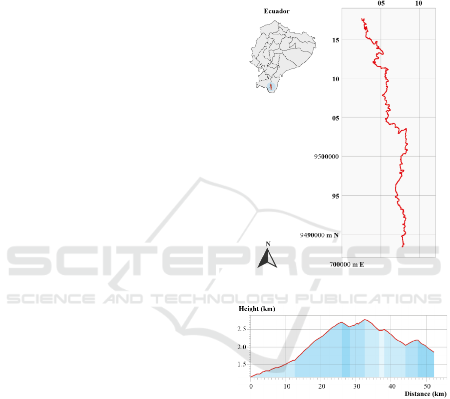
The selected road for the study was in a mountainous
topography (see Figure 1). Considering its geometric
design limitations, this type of road allows it to have
a high number of horizontal curves. Also, combine
them with other geometric elements, such as steep
grades. The evaluated road section has a length of
more than 50 km. The longitudinal profile of the road
is shown in Figure 2. In this profile, the sections with
homogeneous grades have been shaded. This profile
was obtained from the GPS data of the VBOX tool.
The selected road is located in the Ecuadorian
Amazon between Palanda and Yangana town. This
road belongs to the "Eje Vial No. 4" that
communicates Ecuador with Peru. The road has a
rigid pavement roadway and has a lane width of 3.65
m. The road crosses several protected forests:
Podocarpus National Park and Tapichalaca Reserve.
The mountain forests and paramos of the region are
considered "super-humid" since rainfall over 6000
mm has been recorded (Richter, 2003).
Figure 1: Planimetry of the selected road for this
experimental study (Ecuador).
Figure 2: Road vertical profile of the selected road.
2.2 Test Vehicle Selection
The vehicle selected was a Chevrolet D-Max diesel
pickup. The truck has the characteristics shown in
Table 1. This car is practical in the case of small
landslides, small rock falls, among others, which are
frequently on these roads. The vehicle has ABS +
EBD brakes, traction control, and stability control.
2.3 Measurement Tool
The selected measurement tool was the Video VBOX
Lite. This device collects the following data: time,
Real Driving on Under-inflated Rear Tire on Horizontal Curves: A Road Experimental Study
325
distance, satellites, speed (km/h), heading (degrees),
latitude, longitude, height (m), vertical velocity
(km/h), longitudinal and lateral acceleration (m/s²).
Table 1: Technical specifications of the test vehicle.
Characteristic Condition
Motor 2,5L turbo diesel
Net Power (Hp @ rpm) 34 @ 3600
Torque (Nm @ rpm) 320 @ 1800
Traction 4x4
Front suspension
Independent Double
Wishbone Type
Rear suspension Rigid with Crossbow
Gross vehicle weight (kg) 2950
Front axle capacity (kg) 1350
Rear axle capacity (kg) 1870
Tire size 245/75/ R16
Rated press 30 psi
Height (mm) 1790
Width (mm) 1860
Length (mm) 5295
It allows recording geo-referenced digital images
through high-resolution cameras and the GPS
antenna. The antenna was placed on the roof of the
vehicle. The Video VBOX Lite has an accuracy of
0.05% for distance travelled, 0.2 km / h for speed, and
± 10 m for height. Accuracy acceleration: 0.50%
(resolution = 0.01 g and max = 20 g). The device has
a sampling frequency of 10 Hz.
2.4 Road Geometric Design Estimation
The VBOX Lite also collects the heading data. This
variable helped to estimate the horizontal geometry of
the road. The use of heading direction for recreating
the horizontal alignment of an existing road
(Camacho-Torregrosa et al., 2015) is well extended in
the field. The heading remains constant when
traveling along a tangent and varies its slope when
traveling along a horizontal curve. After this
procedure, a check of the radii of the curves was
carried out using the calculation method based on
three known points. With this procedure, 327
horizontal curves were determined. This value means
that there are 6.29 curves per kilometre. The radii of
these curves were between 20 to 558 m.
On the other hand, to determine the grades of the
section, the total length was divided into sub-sections
that have the same slope. In these homogeneous sub-
sections, the average slopes of each section were: -
9%, -8%, -7%, 2%, 4%, 5% and 8%.
2.5 Data Collection Procedure
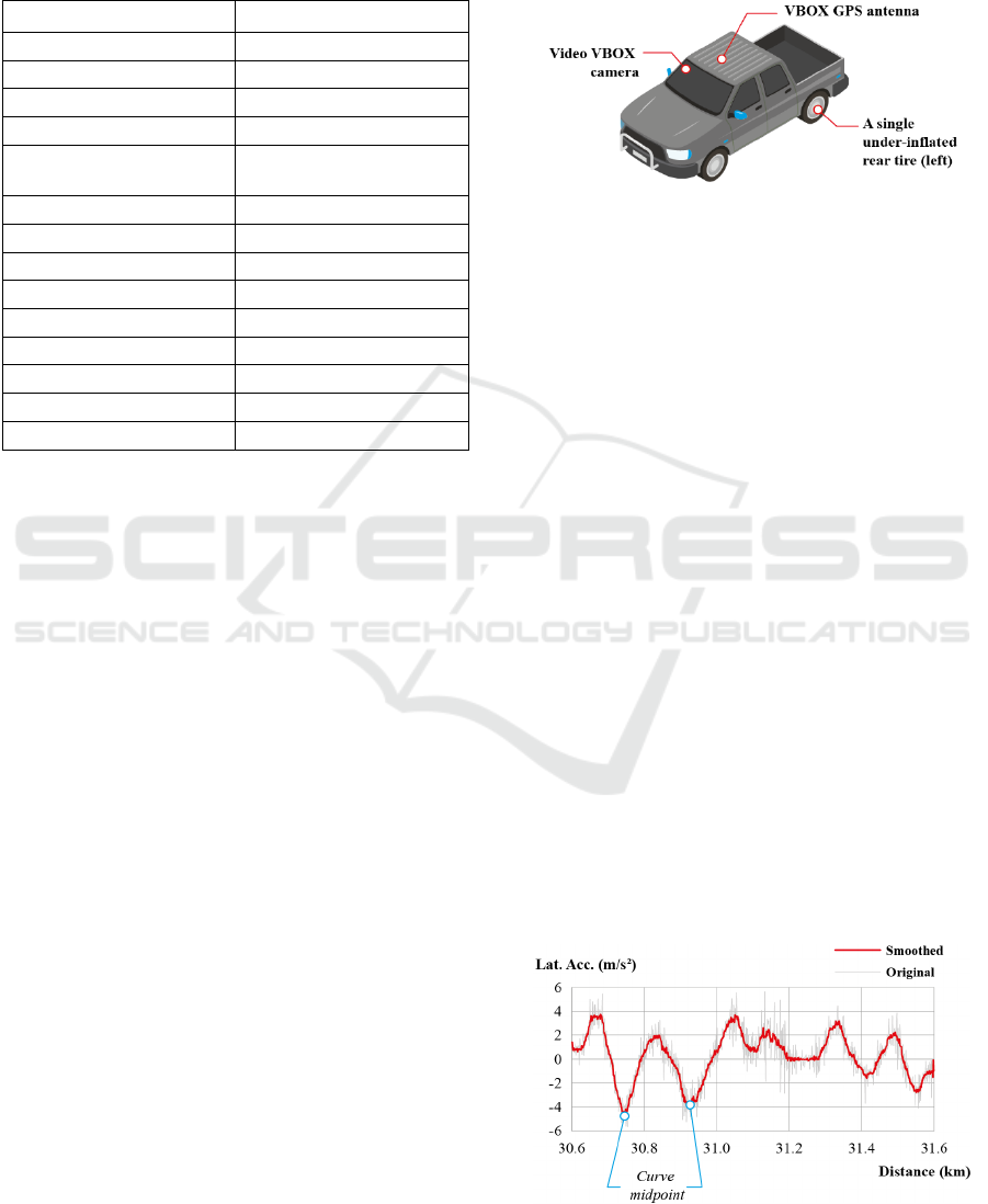
The Video VBOX Lite was placed inside the test
vehicle, as seen in Figure 3. The device has a GPS
antenna and a high-resolution camera.
Figure 3: Details of data collection on the test vehicle.
The antenna was placed in the central part of the
vehicle roof, and the camera was placed on the front
windshield facing the road. Data were collected in
poor weather conditions: light rain, wet pavement,
and daylight. The test vehicle was unloaded. The
rated press of the tire suggested by the manufacturer
in the unloaded state is 30 psi. The air pressure of the
left rear tire was reduced to 10 psi. This value was
taken from the previous literature (Robinette et al.,
1997). A single trip was made considering the risk of
the test. As a precaution, emergency and mechanical
units were located in the middle and end of the route.
After finishing the experiment, the mechanical team
checked the tire and the operation of the entire vehicle
and its components. During the test, the driver was
always able to easily maintain control of the test
vehicles and steer them in the road test.
2.6 Data Processing
After the data collection, video and data were
obtained employing the VBOX Test Suite ® of the
equipment manufacturer. It eliminated all the
following data: the vehicle was not in free flow,
overtaking maneuverer, in an urban or suburban area,
or when the road deteriorated. The acceleration data
were subjected to a smoothing process using a
Figure 4: Example of lateral acceleration smooth.
VEHITS 2022 - 8th International Conference on Vehicle Technology and Intelligent Transport Systems
326
moving average with a window width of 7. Figure 4
shows as an example, the original and smoothed
profile of lateral acceleration. After this procedure,
the data was extracted in the midpoint of the
horizontal curve, also shown in Figure 4.
3 RESULTS
The number of satellites registered on the route was
between 6 and 13, with an average of 10. The
minimum speed was 5.03, and the maximum was
69.37 km/h. Previous studies reached 72 km/h
(Robinette et al., 1997). The under-inflated rear tire
could mainly affect the speed, vertical velocity,
longitudinal acceleration, and lateral acceleration. It
would have very little relevance to analyse all the
acceleration values without considering the geometry
of the road. Therefore, these are discussed below for
the road grades and the radii of the curves.
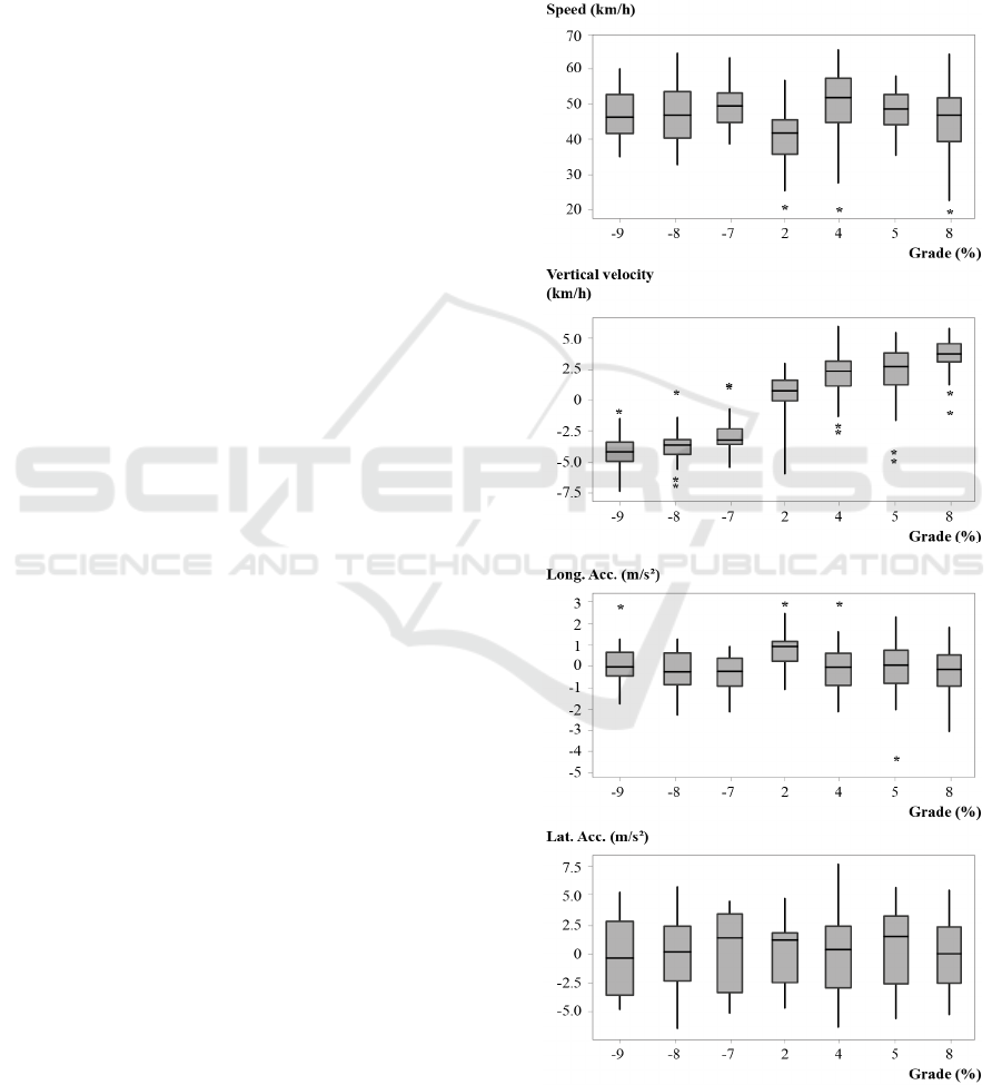
3.1 Road Grades Analysis
In order to analyse the variations of the variables
concerning the grade, the homogeneous sections with
similar slopes were grouped. Then, it calculated their
average grade in every section. Then, it plotted the
boxplots of the speed, vertical velocity, longitudinal
and lateral acceleration versus the grade of the road
(see Figure 5). In Figure 5, it can be seen just the
logical relationship between vertical velocity and
slope. Vertical velocity has a direction associated, is
positive when climbing, and is negative when
descending. Regarding speed, there are no significant
variations between positive or negative slopes that
have been reported in previous research (García-
Ramírez & Alverca, 2019). Previous studies found
higher speeds on descending slopes and lower them
on ascending slopes. This situation could be a result
of a mountain topography with consecutive curves,
where the grade could be less important than the
curvature itself.
3.2 Curve Radii Analysis
The scatterplot of the speed, vertical velocity,
longitudinal and lateral acceleration is seen in Figure
6. The scatterplot of the speed, vertical velocity,
longitudinal and lateral acceleration is seen in Figure
6. In this figure, when the radius of the curve is lower,
speeds go down, and vice versa. This relationship is
well documented in previous speed prediction
models. Regarding the vertical velocity, the Figure 5
does not show any trend with the grade or the radius
of the curve. On the other hand, the longitudinal
acceleration does not present any visible trend, unlike
the lateral acceleration, where the highest values are
found in the radii smallest and the lowest at the largest
radii. This relationship is consistent with the highway
geometric design philosophy (AASHTO, 2011).
In Figure 6, the direction of the curve has also
been placed. This was done because the driver, during
Figure 5: Boxplot of speed, vertical velocity, longitudinal
and lateral acceleration versus the grade of the road.
Real Driving on Under-inflated Rear Tire on Horizontal Curves: A Road Experimental Study
327
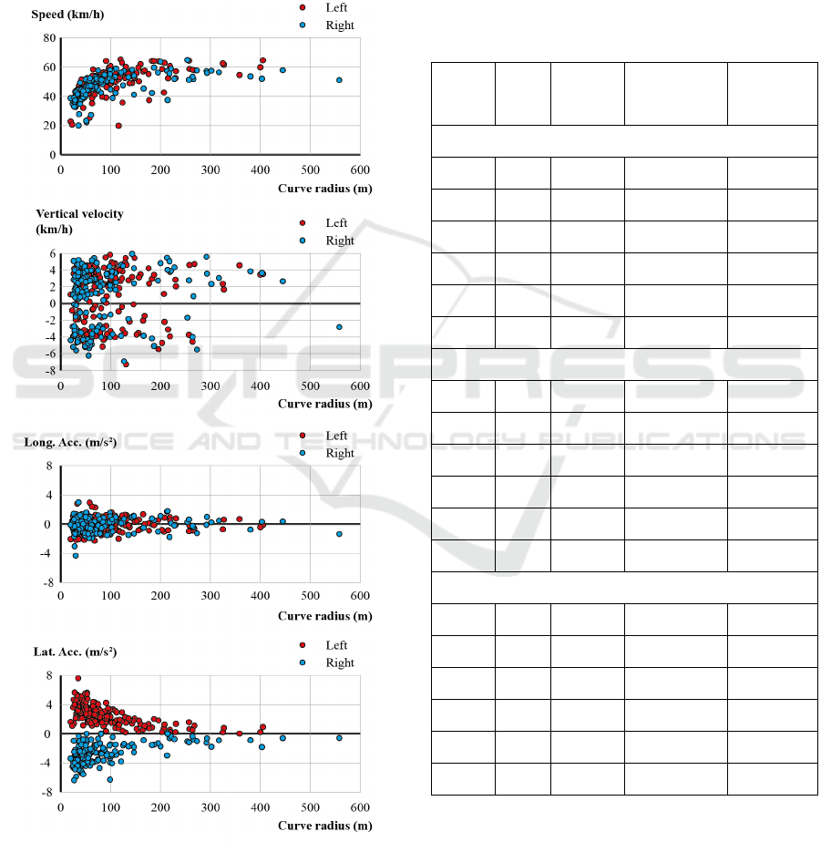
the test, reported skidding in the left curves. The
grade and vertical speed were discarded since there
were no significant differences. Table 2 shows the
average speed, acceleration, and radius. This table
confirmed the trends in Figure 6, and, other two
interesting elements appear, the speeds generally are
lower in the right curves; while the lateral
accelerations are lower in those curves. In the next
section, this element will be analysed in deep.
Figure 6: Scatterplot of the speed, longitudinal and lateral
acceleration versus the radius of the curve and considering
the direction of the curve.
3.3 Descriptive Statistics Analysis
Table 3 presents the descriptive statistics of the
variables previously detected. This table shows the
mean longitudinal acceleration in the right curve is
greater than in the left. The rest of the statistics are
very similar to each other, except for the minimum
value. Regarding the mean lateral acceleration, the
value of the right curve is also greater than the left.
Table 2: Descriptive statistics of speed and acceleration
with the ranges of the radii of the curves.
Radii of
curves
(m)
N
Mean
Speed
(km/h)
Mean long.
acc. (m/s
2
)
Mean lat.
acc. (m/s
2
)
All data
20-50 110 40.1 -0.233 3.518
51-100 123 48.9 -0.145 2.707
101-150 43 52.1 0.188 1.981
151-200 16 55.9 0.090 1.218
201-250 13 54.4 0.155 0.719
>250 22 57.4 -0.151 0.856
Right curves
20-50 66 39.7 -0.242 -3.461
51-100 52 48.0 -0.321 -2.671
101-150 16 51.6 0.144 -2.305
151-200 5 53.4 0.188 -1.382
201-250 5 52.2 0.336 -0.934
>250 13 55.5 -0.057 -0.980
Left curves
20-50 44 40.6 -0.219 3.604
51-100 71 49.5 -0.015 2.735
101-150 27 52.3 0.214 1.790
151-200 11 57.0 0.045 1.143
201-250 8 55.7 0.041 0.585
>250 9 60.2 -0.288 0.677
Regarding the speeds, in general, higher values
were obtained in the left curves than in the right
curves. The driver was expected to slow down in the
right curves since with the under-inflated rear tire, the
possibility of outward skidding was a consequence.
This behaviour does not occur on left curves. This
VEHITS 2022 - 8th International Conference on Vehicle Technology and Intelligent Transport Systems
328

particularity also impacts the lateral acceleration,
since although the left curves have higher average
speeds, they have lower lateral acceleration values
than the right ones. The same happens in longitudinal
acceleration. In conclusion, the presence of an under-
inflated left rear tire impacts a reduction in average
speed in left curves and an increase in average lateral
acceleration and average longitudinal acceleration.
The variations are -6.5%, + 8.5% and + 78% for
speed, lateral acceleration and average longitudinal
acceleration, respectively.
Table 3: Descriptive statistics of speed and acceleration for
the direction of the curve.
Variable
Curve
type
N Mean StDev. Min Max
Long.
acc.
(m/s
2
)
Right
157
-0.182
0.997
-4.320
2.98
Left
170
-0.040
0.942
-2.27
2.94
Lat.
acc.
(m/s
2
)
Right
157
2.729
1.420
0.000
6.360
Left
170
2.496
1.397
0.030
7.590
Speed
(km/h)
Right
157
45.803
8.166
20.110
64.840
Left
170
48.981
8.610
19.940
65.200
3.4 Linear Regression Analysis
Due the differences between the direction of the
curves, the following linear regression analysis was
carried out as shown in Table 4.
The regression analysis was done with the
Stepwise function of Minitab ® (State College,
2005). These equations are referential and should be
explored further in future research.
Table 4 shows the models for all the data, the right
curves, and the left curves. The lateral acceleration
was a dependent variable. The main predictors for
lateral acceleration are: the speed and the radius of the
curve. It used the R
-1
(inverse of the curve radii) in the
regression process, but it was not statistically
significant. The model that best fits is the one for the
Table 4: Linear regression models for the lateral
acceleration and the direction of the curve.
Predictor Coef.
SE
Coef.
T-
value
P-
value
R
2
ad
j
.
All data
Constant -2.20 0.92 -2.39 0.018
1.5
%
Speed
(
km/h
)
0.05 0.02 2.41 0.016
Right curves
Constant -3.49 0.14 -24.96 0.000
26.4
%
Curve
radii
(
m
)
0.09 0.00 7.94 0.000
Left curves
Constant 3.67 0.14 26.37 0.000
39.4
%
Curve
radii (m)
-0.01 0.00 -10.54 0.000
Coef.: model coefficients, SE Coef.: standard error of the
coefficient, T-value: ratio between the coefficient and its
standard error, P-value:
p
robability that measures the
evidence against the null hypothesis, R
2
adj.: adjusted R-
squared.
left curves. This outcome was expected because the
under-inflated tire did not have a meaningful effect on
these curves. The real impact is in the right curves,
where the coefficient of determination is low. And
this also affects the fit of the general model, so the R
2
adjusted is very low.
4 CONCLUSIONS
This article aimed to investigate the influence on the
stability variables of the vehicle in curves of the road
when the vehicle driving on the under-inflated rear
tire on wet pavement. After analysing the results, the
following conclusions are presented:
The speed and acceleration were the variables that
were mainly affected because of a left under-inflated
rear tire. However, the influence was only present in
curves on the opposite side of the under-inflated rear
tire. Speed decreases in these curves, while lateral
acceleration increases. The radius of the curve was
also statistically significant; nevertheless, the grade of
the road was not. That is why equations were
calibrated with this variable, where, as a result of the
presence of the under-inflated tire, the right curves
had less regression fit than the left curves. It is
necessary to mention that differences in lateral
acceleration in left or right curves are not only to the
flat tire but it could also have been caused by the
driver, for whom a left curve differs from a right
Real Driving on Under-inflated Rear Tire on Horizontal Curves: A Road Experimental Study
329

curve since he/she sits on one side of the vehicle. This
could be analysed in future studies.
This study has several limitations. First, this study
employed a single vehicle and a single under-inflated
rear tire. Additionally, just one trip was conducted in
the experiment, with 10-psi tire pressure. Both
conditions could differ in other vehicles, another tire
or air pressure, or driving several trips. It did not
repeat the trip due to an accident hazard. It would be
interesting to compare at least 3 cases: 1) current case,
2) normal case (all tires inflated to 30 psi) 3) the right
rear tire reduced to 10 psi, and other combinations.
This study focused on the kinematics effects of an
under−inflated tyre; therefore, we don’t know what
are the causes of this behaviour: rolling resistance, the
contact area tyre, among others. These causes could
be modelled as seen in Varghese (2013). With this
procedure, it could predict the effect of more
under−inflated tires and complement the presented
experiment that involves only one under−inflated tire.
Despite these limitations, the present study helps
to extend the knowledge of the consequences of an
under-inflated rear tire, and their relationship with the
road geometric variables. Data in this study belonged
to the actual driving on more than 50 km in the
mountainous road. This context was not previously
analysed. Although modern vehicles include direct
monitoring of the tire pressure, the present outcomes
can be the basis for a new indirect pressure method in
accidents reconstructions, which can be analysed in
future studies.
ACKNOWLEDGEMENTS
The author acknowledges the support of the National
Secretariat of Higher Education, Science,
Technology and Innovation (SENESCYT) and
Universidad Técnica Particular de Loja from the
Republic of Ecuador.
REFERENCES
AASHTO. (2011). A policy on geometric design of
highways and streets. American Association of State
Highway and Transportation Officials.
Camacho-Torregrosa, F. J., Pérez-Zuriaga, A. M., Campoy-
Ungría, J. M., García, A., & Tarko, A. P. (2015). Use
of Heading Direction for Recreating the Horizontal
Alignment of an Existing Road. Computer-Aided Civil
and Infrastructure Engineering, 30(4), 282–299.
https://doi.org/10.1111/MICE.12094
Fancher, P. S., Bernard, J. E., & Emery, L. H. (1974). The
effects of tire-in-use factors on passenger car
performance. SAE Technical Papers. https://doi.org/
10.4271/741107
García-Ramírez, Y. D., & Alverca, F. (2019). Calibración
de Ecuaciones de Velocidades de Operación en
Carreteras Rurales Montañosas de Dos Carriles: Caso
de Estudio Ecuatoriano. Revista Politécnica, 43(2), 37–
44. https://doi.org/10.33333/rp.vol43n2.1012
Goharimanesh, M., Riahi, A., Lashkaripour, A., & Akbari,
A. A. (2016). Tire inflation pressure estimation using
identification techniques. International Journal of
Software Engineering and Its Applications, 10(7), 135–
144. https://doi.org/10.14257/IJSEIA.2016.10.7.13
Liqiang, W., Lin, Q., Zhe, Z., & Zongqi, H. (2018).
Research on the compensation method of Indirect Tire
Pressure Monitoring under Sinusoidal Driving
Condition. MATEC Web of Conferences.
https://doi.org/10.1051/matecconf/201815304007
Motrycz, G., Helnarska, K. J., & Stryjek, P. (2021).
Continuing a vehicle fitted with run flat tyres. Scientific
Journal of Silesian University of Technology. Series
Transport, 112, 157–169. https://doi.org/10.20858/
SJSUTST.2021.112.7.13
Pacejka, H. (2012). Tire and Vehicle Dynamics. In Tire and
Vehicle Dynamics (3th ed.). Elsevier Ltd.
https://doi.org/10.1016/C2010-0-68548-8
Richter, M. (2003). Using epiphytes and soil temperatures
for eco-climatic interpretations in southern Ecuador.
Erdkunde, 57(3), 161–181. https://doi.org/10.3112/
ERDKUNDE.2003.03.01
Robinette, R., Deering, D., & Fay, R. J. (1997). Drag and
steering effects of under inflated and deflated tires. SAE
Technical Papers. https://doi.org/10.4271/970954
State College. (2005). Minitab 14.2 Statistical Software
[Computer program] (14.2). PA: Minitab, Inc.
www.minitab.com
Toma, M., Andreescu, C., & Stan, C. (2018). Influence of
tire inflation pressure on the results of diagnosing
brakes and suspension. Procedia Manufacturing, 22,
121–128.
https://doi.org/10.1016/J.PROMFG.2018.03.019
Varghese, A. (2013). Influence of Tyre Inflation Pressure
on Fuel Consumption, Vehicle Handling and Ride
Quality. Chalmers University of Technology [Master’s
thesis].
Zebala, J., & Wach, W. (2014). Lane change maneuver
driving a car with reduced tire pressure. SAE Technical
Papers,
1. https://doi.org/10.4271/2014-01-0466
Zȩbala, J., Wach, W., Ciȩpka, P., & Janczur, R. (2014). Car
motion with reduced tire pressure - Experiment vs.
simulation. Z Zagadnien Nauk Sadowych, 97, 34–47.
VEHITS 2022 - 8th International Conference on Vehicle Technology and Intelligent Transport Systems
330
