The Subtle Art of Digging for Defects: Analyzing Features for Defect

Prediction in Java Projects

Geanderson Santos

, Adriano Veloso

and Eduardo Figueiredo

Universidade Federal de Minas Gerais, Belo Horizonte, Brazil

Keywords:

Defect Prediction, Software Features for Defect Prediction, Machine Learning Models.

Abstract:

The task to predict software defects remains a topic of investigation in software engineering and machine

learning communities. The current literature proposed numerous machine learning models and software fea-

tures to anticipate defects in source code. Furthermore, as distinct machine learning approaches emerged in

the research community, increased possibilities for predicting defects are made possible. In this paper, we dis-

cuss the results of using a previously applied dataset to predict software defects. The dataset contains 47,618

classes from 53 Java software projects. Besides, the data covers 66 software features related to numerous

aspects of the code. As a result of our investigation, we compare eight machine learning models. For the

candidate models, we employed Logistic Regression (LR), Naive Bayes (NB), K-Nearest Neighbor (KNN),

Multilayer Perceptron (MLP), Support Vector Machine (SVM), Decision Tree (CART), Random Forest (RF),

and Gradient Boosting Machine (GBM). To contrast the models’ performance, we used ﬁve evaluation metrics

frequently applied in the defect prediction literature. We hope this approach can guide more discussions about

benchmark machine learning models for defect prediction.

1 INTRODUCTION

With the consistent expansion of software develop-

ment, the reliability of these projects represents a key

concern for developers and stakeholders alike (Jing

et al., 2014; Wang et al., 2016). The software sys-

tems’ internal features and capabilities may introduce

defects leading the software project to fail in various

stages of development and maintenance. Guided by

this matter, software teams adopt strategies to miti-

gate the impacts of defective code. As a result, the

current literature reports several efforts to assist de-

velopers to anticipate future defects in the source code

(Nagappan et al., 2006; Hassan, 2009; D’Ambros

et al., 2010; Tantithamthavorn et al., 2019). As an

example, software defect prediction is one of the re-

search directions in applying machine learning mod-

els to predict software defects in projects. In this do-

main, prior studies investigated code metrics as pre-

dictors of software defects (Nagappan et al., 2006;

Menzies et al., 2007; Moser et al., 2008; Menzies

et al., 2010; D’Ambros et al., 2010; dos Santos

https://orcid.org/0000-0002-7571-6578

https://orcid.org/0000-0002-9177-4954

https://orcid.org/0000-0002-6004-2718

et al., 2020) and bad smells (Khomh et al., 2012;

Palomba et al., 2013). This cooperation is strengthen-

ing as both software engineering and machine learn-

ing ﬁelds become closer in the task of anticipating de-

fects in source code (Tantithamthavorn et al., 2019;

Jiarpakdee et al., 2020; dos Santos et al., 2020).

Corresponding to the software features to pre-

dict defects, various studies focus on unique fea-

tures extracted from source code that may cause

defects (Nagappan et al., 2006; Amasaki, 2018).

For instance, these software features could represent

change metrics (Moser et al., 2008; D’Ambros et al.,

2010), class-level metrics (Herbold, 2015; Jureczko

and Madeyski, 2010), Halstead and McCabe met-

rics (Menzies et al., 2007; Menzies et al., 2010), en-

tropy metrics (Hassan, 2009; D’Ambros et al., 2010),

among others. In this paper, we do not differentiate

software features from code metrics. Despite the ad-

vantages of using such software features to predict

defects, one issue is that the machine learning mod-

els are not always useful for the software community.

As a result, one of the main challenges faced by re-

searchers is the applicability of these models in real-

world projects (Ghotra et al., 2015). To tackle this

problem, we focus on data analysis of a large dataset

known as uniﬁed dataset (Ferenc et al., 2018; Ferenc

Santos, G., Veloso, A. and Figueiredo, E.

The Subtle Art of Digging for Defects: Analyzing Features for Defect Prediction in Java Projects.

DOI: 10.5220/0011045700003176

In Proceedings of the 17th International Conference on Evaluation of Novel Approaches to Software Engineering (ENASE 2022), pages 371-378

ISBN: 978-989-758-568-5; ISSN: 2184-4895

371

et al., 2020a). This data contains information about

47,618 classes, 53 Java projects, and 66 software fea-

tures. These software features relate to different char-

acteristics of the code such as cohesion, complexity,

coupling, documentation, inheritance, and size (T

oth

et al., 2016). In contrast to other works from the cur-

rent literature (Jureczko and Spinellis, 2010), the uni-

ﬁed dataset presents numerous features and classes,

which makes the analysis more comprehensive about

the software features.

Furthermore, we applied three steps to ﬁt the data

for the experiments. In the ﬁrst step, we use data

cleaning to deal with missing and duplicate entries.

Second, we apply data normalization, balancing, and

encoding the data. Finally, we use feature engineer-

ing concepts to create new software features from the

existing ones, to select the relevant software features

for the prediction, and to analyze the correlation and

variance of the remaining software features. To com-

pare the results of the data preparation, we use eight

benchmark algorithms to validate the analysis. These

algorithms are largely applied in the defect predic-

tion literature. Our results suggest that three mod-

els are efﬁcient in predicting defects in Java projects.

Random Forest, Gradient Boosting Machine, and K-

Nearest Neighbor.

This paper is organized as follows. Section 2

presents the methodology and its main steps. Thus,

we discuss the goals and the research question that

guided the investigation (Section 2.1). Next, we

present the data (Section 2.2) and the data prepara-

tion (Section 2.3). Moreover, we present the software

features (Section 2.4). Then, Section 3 discusses the

main results of our paper. Next, Section 4 presents

the threats to validity of our study. In Section 5, we

present some relevant work related to our paper. Fi-

nally, Section 6 discusses the ﬁnal remarks and further

explorations of our paper.

2 METHODOLOGY

This section describes the methodology we choose

to investigate the software defects in Java projects.

We divide our method into four steps. Section 2.1

presents the main goal and research questions from

our experiments. Next, we discuss the dataset we used

to predict software defects (Section 2.2). Then, Sec-

tion 2.3 displays the data preparation applied to ﬁt the

data for the experiments. Afterward, Section 2.4 de-

scribes the software features for defect prediction in

Java projects that we extracted from the entire set of

software features.

2.1 Goal and Research Questions

In this paper, we investigate different algorithms that

may explain the software features that contribute to

the defectiveness of Java classes. To do so, we em-

ployed data preparation to ﬁnd the software features

for the defect prediction task and to clean the data.

Therefore, our main objective is to investigate soft-

ware features applied for defect prediction. Guided

by this objective, our paper examines the following

overarching question.

− How effective are benchmark models to the defect

prediction task in Java projects?

To explore this research question, we rely on a pre-

viously used dataset about defect prediction (Ferenc

et al., 2018; Ferenc et al., 2020a). This dataset con-

veys information about 53 Java projects and 66 soft-

ware features. After cleaning and exploring the data,

we compare the accuracy of benchmark models previ-

ously applied in the literature. We compare ﬁve evalu-

ation metrics: ROC Area Under the Curve (AUC), F1

score, precision, recall, and accuracy. For the candi-

date models, we employed Logistic Regression (LR),

Naive Bayes (NB), K-Nearest Neighbor (KNN), Mul-

tilayer Perceptron (MLP), Support Vector Machine

(SVM), Decision Tree (CART), Random Forest (RF),

and Gradient Boosting Machine (GBM). Our research

provides intriguing discussions about machine learn-

ing models for defect prediction. For instance, we

show that RF, GBM, and KNN are slightly more ef-

fective in predicting defects in Java classes (over 90%

of AUC compared to other classiﬁers).

2.2 Uniﬁed Data

The dataset used in our experiments represents a

merged version of several resources available for the

scientiﬁc community (T

oth et al., 2016; Ferenc et al.,

2018; Ferenc et al., 2020a; Ferenc et al., 2020b). In

total, ﬁve data sources provided the data: PROMISE

(Sayyad S. and Menzies, 2005), Eclipse Bug Pre-

diction (Zimmermann et al., 2007), Bug Prediction

Dataset (D’Ambros et al., 2010), Bugcatchers Bug

Dataset (Hall et al., 2012), and GitHub Bug Dataset

oth et al., 2016)

. The dataset contains 47,618

classes from 53 Java projects. Furthermore, the data

comprises 66 software features related to different as-

pects of the code. More details about the dataset and

the models generated in this paper are available in the

replication package

. The dataset is imbalanced as

https://zenodo.org/record/3693686

https://github.com/anonymous-replication/replication-

package-uniﬁed

ENASE 2022 - 17th International Conference on Evaluation of Novel Approaches to Software Engineering

372

only around 20% of the classes represent a software

defect (Ferenc et al., 2018). For this reason, we had

to apply a data preparation step to create the machine

learning models to predict software defects as we dis-

cuss next.

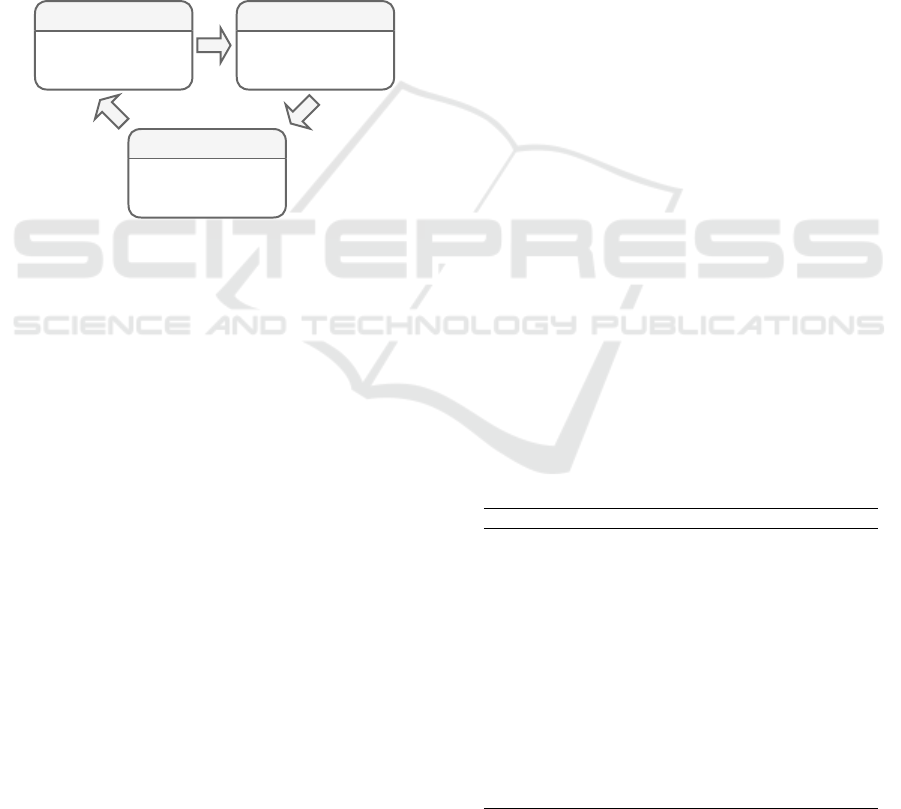
2.3 Data Preparation

To prepare the data for the experiments, we needed

to apply several machine learning processes. Figure

1 exempliﬁes the data preparation executed in our pa-

per. These steps were necessary not only to clean the

data and avoid misinterpretation but also to discover

a list of software features picked during the feature

selection step.

(i) (ii)

(iii)

DataCleaning

-Non-numericdata

-RemoveDuplicates

-MissingValues

DataExploration

-Normalization

-Balancing

-Encoding

FeatureEngineering

-FeatureSelection

-Correlation-Threshold

-VarianceAnalysis

Figure 1: Data Preparation Process.

Data Cleaning. First, we applied data cleaning to

eliminate duplicated classes and non-numeric data (i -

Figure 1). This process is especially critical in the de-

fect prediction task, as many datasets have incorrect

entries gathered by automatic systems (Petri

c et al.,

2016). We execute data imputation to track the miss-

ing values. At the end of this step, we could reduce

the dimension of the data as we remove repeated data

entries.

Data Exploration. Further, in the second step of the

data preparation (ii - Figure 1), we executed data ex-

ploration. Here, we track over-represented features,

applied one-hot encoding (Lin et al., 2014), and nor-

malize the data. At last, we removed two software

features in the over-represented step. These software

features gathered information about the exact line of

code a class started and ﬁnished. In terms of encod-

ing, we applied one-hot encoding to the type feature.

The type feature stored information about the class

type. For instance, we created new features for class,

enumerates, interfaces, and annotations. Since we

are aware of the multicollinearity problem that one-

hot encoding may introduce in the models, we tested

for Variance Inﬂation Factor (VIF), and we concluded

that the preparation was done right (low VIF values).

Finally, we applied data normalization using Standard

Scaler, and Synthetic Minority Oversampling Tech-

nique (SMOTE) (Tantithamthavorn et al., 2018) to

deal with the imbalanced nature of the dataset. In

total, the uniﬁed data contained only around 20% of

defective classes. For this reason, oversampling was

necessary to generate models that could generalize to

unseen data.

Feature Engineering. At the ﬁnal step, we ap-

plied feature engineering to select the features that

are important for our predictions (iii - Figure 1). We

tested several methods to choose the software fea-

tures, although a recent implementation of the Gradi-

ent Boosting Machine known as LightGBM demon-

strated better results in terms of selecting features. At

the end of this process, we ended up with 14 software

features varying from different software characteris-

tics.

2.4 Software Features

The current literature has a plethora of software

features to predict defects (Jing et al., 2014; Tan-

tithamthavorn and Hassan, 2018). The complete list

of features used in the target data (66 in total) is avail-

able under the replication package. Table 1 presents

the fourteen software features selected with the fea-

ture selection step executed in step 2 (Figure 1). Table

1 presents the acronym and name of each of the se-

lected features. All these software features are from

the class-level, due to their scope. As we may ob-

serve, most features are related to size (NA, NG,

NLG, NS, and TNM) (Ferenc et al., 2018). However,

some features are related to documentation (CLOC,

CK, AD, PUA), code coupling (CBOI, NOI), and

code complexity (CC, WMC, NL) (T

oth et al., 2016;

Ferenc et al., 2018).

Table 1: Selected Class Level Software Features.

Acronym Description

WMC Weighted Method per Class

NL Nesting Level

CC Clone Coverage

CBOI Coupling Between Objects classes Inv.

NOI Number of Outgoing Invocations

AD API Documentation

CD Comment Density

CLOC Comment Lines of Code

PUA Public Undocumented API

NA Number of private attributes

NG Number of getters

NLG Number of local getters

NS Number of setters

TNM Total Number of Methods

The Subtle Art of Digging for Defects: Analyzing Features for Defect Prediction in Java Projects

373

3 EXPERIMENTAL RESULTS

This section presents the experimental results of our

paper. First, we discuss the predictive accuracy of the

machine learning models. As a result, we divide the

ﬁrst section into nine parts where the ﬁrst eight in-

troduce the results of the classiﬁcation experiments.

Hence, the last section proposes a discussion of the

experiments. Finally, we present the implications of

our work for the defect prediction task.

3.1 Predictive Accuracy

The predictive accuracy of machine learning mod-

els depends on the association between the structural

software properties and a binary outcome. In this

case, the properties are the software features widely

applied in the literature (Ferenc et al., 2018; Ferenc

et al., 2020a). Therefore, the binary outcome is the

feature that yields the defective or clean class. In

this case, the low association between the software

features and the classiﬁcation technique can generate

a large error. Next, we discuss the predictive accu-

racy of these methods for the target data. To test the

models, we apply ﬁve evaluation metrics (accuracy,

recall, precision, F1, and AUC). The following dis-

cussion takes into consideration the maximum, mini-

mum, median, mean, and standard deviation (SD) of

each evaluation metric.

3.1.1 Logistic Regression

Rows of Table 2 indicate the ﬁve performance met-

rics we used in this study. The columns show their

maximum (Max) and minimum (Min) values. Table

2 also shows the median (Median) and mean (Mean)

and standard deviation (SD) of the performance met-

rics. Table 2 presents the performance of Logistic Re-

gression (LR). In general, LR showed an AUC num-

ber of nearly 77% (on average). Furthermore, the

model using LR is stable as the tradeoff between the

precision and recall is minimum. As we balance the

dataset prior prediction (with oversampling applying

the SMOTE technique), we can consider the AUC

numbers as a good indication of model performance.

In this case, LR is a fair predictor; however, the av-

erage AUC is not optimal (around 77%) compared to

other classiﬁcation models.

3.1.2 Naive Bayes

In Table 3, we can observe that the Naive Bayes (NB)

predictor achieved AUC numbers close to 74%. This

result is lower than the LR model (by approximately

Table 2: Logistic Regression Evaluation.

Max Min Median Mean SD

accuracy 0.701 0.685 0.694 0.693 0.005

recall 0.691 0.668 0.680 0.680 0.009

precision 0.706 0.690 0.698 0.698 0.006

f1 0.698 0.680 0.690 0.689 0.006

roc auc 0.771 0.759 0.769 0.767 0.004

3.5%). Thus, we note that NB shows a high differ-

ence between the F1 and AUC scores. It happens be-

cause the model achieved low recall. It means that

the NB model is demanding and does not think many

classes have defects. All the software classes that are

not defects are undeniably clean (i.e., non-defective).

However, this model misses a lot of actual defects.

We derive this conclusion from the high difference be-

tween precision and recall (around 45%). Although,

this model is also stable as we note by the SD (last

column of Figure 3).

Table 3: Naive Bayes Evaluation.

Max Min Median Mean SD

accuracy 0.614 0.606 0.610 0.610 0.003

recall 0.329 0.314 0.319 0.320 0.005

precision 0.782 0.754 0.758 0.762 0.009

f1 0.460 0.443 0.451 0.451 0.005

roc auc 0.747 0.733 0.741 0.740 0.004

3.1.3 K-Nearest Neighbor

Table 4 shows the results of applying the K-Nearest

Neighbor (KNN) algorithm. We can observe that

the average AUC number is around 91%, the highest

number compared to Logistic Regression and Naive

Bayes. However, this model does not present the high

precision and low recall problem. The difference be-

tween the AUC and F1 is minimum. Another intrigu-

ing result relates to the recall number, which was the

best metric in this model. It means that this model can

select the correct number of defective classes in 94%

of the time. Moreover, the variation denoted by the

SD is also low such as in the previous cases.

Table 4: K-Nearest Neighbor Evaluation.

Max Min Median Mean SD

accuracy 0.842 0.832 0.838 0.838 0.003

recall 0.941 0.928 0.933 0.934 0.005

precision 0.790 0.774 0.784 0.784 0.005

f1 0.856 0.848 0.852 0.852 0.002

roc auc 0.914 0.905 0.909 0.910 0.003

3.1.4 Multilayer Perceptron

Table 5 presents the general performance of using a

Multilayer Perceptron (MLP). The model exhibits a

low variation in their performance, as we observe by

ENASE 2022 - 17th International Conference on Evaluation of Novel Approaches to Software Engineering

374

the SD of all metrics. Like the K-Nearest Neighbor

model, the MLP model showed an efﬁcient classiﬁca-

tion power (AUC numbers of nearly 85%). Further-

more, the F1 score was also high (around 76%). Thus,

the MLP model is consistent in predicting defects in

Java classes, although KNN presented a better perfor-

mance overall.

Table 5: Multilayer Perceptron Evaluation.

Max Min Median Mean SD

accuracy 0.769 0.759 0.764 0.764 0.004

recall 0.790 0.747 0.760 0.763 0.015

precision 0.772 0.747 0.763 0.762 0.008

f1 0.770 0.753 0.764 0.762 0.006

roc auc 0.847 0.835 0.842 0.842 0.003

3.1.5 Support Vector Machine

In Table 6, we show the overall performance of apply-

ing Support Vector Machine (SVM) in the selected

data. As we can observe, this model is very consis-

tent in predicting defective classes in the target lan-

guage. As not only the AUC numbers (approximately

80%) are high, but also the F1 score (nearly 74%)

is high. The model is similar to Logistic Regres-

sion, Multilayer Perceptron, and K-Nearest Neighbor

in that manner (showed a consistent F1 score). How-

ever, KNN is the only model to predict a defect with

above 90% accuracy (measured by AUC), and SVM

falls into the MLP predictive power (where the model

achieved above 80% of AUC).

Table 6: Support Vector Machine Evaluation.

Max Min Median Mean SD

accuracy 0.738 0.725 0.733 0.732 0.004

recall 0.757 0.735 0.746 0.748 0.007

precision 0.733 0.719 0.723 0.725 0.005

f1 0.742 0.728 0.738 0.736 0.005

roc auc 0.809 0.793 0.802 0.802 0.005

3.1.6 Decision Trees

Table 7 displays the results of applying the Decision

Tree (DT) algorithm. We observe that DT is as consis-

tent as Logistic Regression, Support Vector Machine,

Multilayer Perceptron, and K-Nearest Neighbor. The

average AUC number was nearly 86%. As a result,

the model correctly predicts a defect in over 85% of

the cases. In this case, both MLP and SVM present

similar ﬁndings (over 80% accuracy). The F1 score is

very tight to the AUC evaluation metric meaning that,

the machine learning model can predict the classes

that are not defective (speciﬁcity of the model).

Table 7: Decision Tree Evaluation.

Max Min Median Mean SD

accuracy 0.857 0.843 0.850 0.850 0.004

recall 0.860 0.834 0.844 0.845 0.006

precision 0.860 0.848 0.854 0.854 0.005

f1 0.853 0.844 0.848 0.848 0.003

roc auc 0.86 0.847 0.853 0.854 0.004

3.1.7 Random Forest

Table 8 illustrates the performance of Random Forest

(RF). The algorithm achieved accuracy numbers mea-

sured by AUC close to 96%. Compared to other mod-

els, RF achieved very high accuracy numbers. Not

only the AUC numbers are high but also the F1 score

(nearly 90% of F1 measure). For this reason, we con-

sider RF very robust to predict software defects in

Java. The model was the most stable among the an-

alyzed models (SD of around 0.015%). Furthermore,

RF and KNN are the only models to achieve an AUC

number above 90%.

Table 8: Random Forest Evaluation.

Max Min Median Mean SD

accuracy 0.905 0.892 0.900 0.900 0.004

recall 0.903 0.889 0.897 0.896 0.005

precision 0.910 0.896 0.898 0.900 0.005

f1 0.904 0.893 0.899 0.899 0.004

roc auc 0.956 0.95 0.955 0.954 0.003

3.1.8 Gradient Boosting Machine

In Table 9, we show the performance of the Gradi-

ent Boosting Machine (GBM). The model achieved

an AUC number of nearly 95%. For this reason, GBM

falls into the K-Nearest Neighbor and Random Forest

categories, where these models reached above 90% of

predictive power. Furthermore, the model is stable in

terms of presenting a very low SD. The model is ro-

bust as the F1 score is close to 88%.

Table 9: Gradient Boosting Machine Evaluation.

Max Min Median Mean SD

accuracy 0.890 0.876 0.883 0.883 0.003

recall 0.846 0.825 0.835 0.835 0.005

precision 0.932 0.915 0.923 0.923 0.004

f1 0.885 0.869 0.877 0.877 0.004

roc auc 0.954 0.944 0.949 0.949 0.002

3.1.9 Discussion

Table 10 shows the overall performance of all bench-

mark machine learning models. We observe that

Random Forest (RF) and Gradient Boosting Machine

(GBM) show the highest AUC numbers. RF also

showed the highest F1 score and accuracy numbers.

The Subtle Art of Digging for Defects: Analyzing Features for Defect Prediction in Java Projects

375

In terms of precision, i.e., the number of chosen de-

fective classes that are correctly selected by the ma-

chine learning model, the GBM demonstrated better

results than the other models. It is intriguing to note

that the K-Nearest Neighbor (KNN) showed the best

recall score, i.e., the percentage of correct defective

classes that were selected by the model.

Table 10: Overall Performance of Benchmark Models.

accuracy recall precis. f1 auc

LR 0.693 0.680 0.698 0.689 0.767

NB 0.610 0.320 0.762 0.451 0.740

KNN 0.838 0.934 0.784 0.852 0.910

MLP 0.764 0.763 0.762 0.762 0.842

SVM 0.732 0.748 0.725 0.736 0.802

DT 0.850 0.845 0.854 0.848 0.854

RF 0.901 0.896 0.901 0.899 0.954

GBM 0.883 0.835 0.923 0.877 0.949

Therefore, we conclude that three machine learn-

ing models are more efﬁcient in predicting defects in

Java: GBM, RF, and KNN. Other algorithms did not

perform as well as these models. However, if the de-

veloper is interested in the recall of a model, we rec-

ommended using the KNN algorithm as it showed the

best performance for that evaluation metric. Overall,

GBM is the most consistent model as it represents the

lowest variance among the selected benchmark mod-

els.

The results suggested that ensemble meth-

ods, such as RF and GBM, tend to perform

slightly better at predicting defects for the tar-

get dataset. However, developers interested in

the recall should focus on the KNN model

3.2 Implications

This section presents the main limitations that could

potentially threaten the results of this paper.

− We discovered that three models are more effec-

tive in predicting defects in Java projects: Ran-

dom Forest, Gradient Boosting Machine, and K-

Nearest Neighbor. Further explorations about pre-

dicting defects in Java projects could favor these

machine learning models instead of the other ﬁve

experimented in our investigation.

− The feature engineering technique discovered

fourteen software features from the original 66

features (Table 1). Most features relate to size

(NA, NG, NLG, NS, and TNM) (Ferenc et al.,

2018). However, some features related to docu-

mentation (CLOC, CK, AD, PUA), code coupling

(CBOI, NOI), and code complexity (CC, WMC,

NL) (Ferenc et al., 2020a).

4 THREATS TO VALIDITY

This section presents the main limitations that could

potentially threaten the results in this paper.

− Internal Validity: Threats related to internal va-

lidity are practices that can inﬂuence the indepen-

dent variable to causality (Wohlin et al., 2012). In

this paper, the chosen dataset is a possible threat

to the internal validity, as we naively employed

the data reported in the current literature (Ferenc

et al., 2018). As a result, we cannot reason on data

quality, as any storing process could insert erro-

neous data into the dataset, especially in a com-

plex context such as software development. An-

other problem with the data is the fact that around

80% of the target classes represent non-defective

instances and only around 20% represents defects.

− External Validity: External validity threats are

conditions that limit our ability to generalize the

results of our study (Wohlin et al., 2012). In our

paper, these threats relate to the limited number

of programming languages we investigated. In

this case, we only analyzed the Java programming

language. For this reason, it may be a problem

to generalize the ﬁndings of our paper to distinct

programming languages, especially for languages

that are very unusual from Java.

− Construct Validity: Threats to the construct va-

lidity relate to assuming the result of the exper-

iments to the concept or theory (Wohlin et al.,

2012). The feature engineering technique used in

this paper is a possible threat to the construct va-

lidity. We tested several approaches and decided

to focus on a tree-based technique for feature se-

lection. However, the tree-based may not gener-

alize well to other models. Furthermore, it may

be the reason the tree-based models outperformed

other models, as we derive the set of relevant fea-

tures from them.

− Conclusion Validity: Threats to the conclusion

validity correspond to issues that affect the abil-

ity to dispatch the correct conclusion between the

procedure and the consequence (Wohlin et al.,

2012). Our study, in most parts, depends on

the software features selected in data prepara-

tion. Furthermore, we cannot guarantee how

much distinct feature selection techniques would

differ from the target method.

ENASE 2022 - 17th International Conference on Evaluation of Novel Approaches to Software Engineering

376

5 RELATED WORK

One effort to create effective Machine Learning mod-

els valuable for the Software Engineering community

represents the predictive models using source code

features. These studies share the fact that they use

code metrics for the prediction. Furthermore, they

vary in terms of accuracy, complexity, target program-

ming language, and the input dataset. For instance,

Nagappan and Ball (2005) discuss a technique for

software defect prediction density. Under those cir-

cumstances, they discover a collection of applicable

code churn patterns. The works use regression mod-

els to determine the absolute measures of code churn.

They conclude that these features are poor predictors

of defect density. As a result, they propose a set of

features to predict defect density (Nagappan and Ball,

2005).

In a similar approach, Nagappan et al. (2006) con-

ducted an empirical exploration of the post-release

defect history with ﬁve Microsoft projects. The works

located that some defect-prone features show a high

correlation with code complexity measures. In the

end, they apply principal component analysis on the

code metrics to build regression models that accu-

rately predict the likelihood of post-release defects.

These studies are undoubtedly valuable to the defect

prediction task. However, they do not provide any

insights into the software features’ capacity to inter-

pret the machine learning models (Nagappan et al.,

2006). Similarly, the work of Xu et al. (2018) em-

ployed a non-linear mapping method to extract repre-

sentative features by embedding the initial data into a

high-dimension space (Xu et al., 2018).

In these lines, Wang et al. (2016) examined the

impact of using the program’s semantic on the pre-

diction model’s features. This study tests ten open-

source projects, and it improved the F1 score for both

within-project defect prediction by 14.2% and cross-

project defect prediction by 8.9%, compared to con-

ventional features. The works used deep belief net-

works to automatically learn semantic features from

token vectors obtained from abstract syntax trees

(Wang et al., 2016). Another tackle into the defect

prediction came from Jiang et al. (2013). This study

proposed a personalized defect prediction technique

for each developer. The works use software features

composed of attributes extracted from a commit, such

as Lines of Code (LOC). The study used three types

of software features, namely vectors, bag-of-words,

and metadata information (Jiang et al., 2013).

6 CONCLUSION

This work presented the evaluation of eight different

algorithms employed to predict software defects in

Java projects. We measure the performance of the al-

gorithms on a dataset recently published that encapsu-

lates several years of development in 53 Java projects.

In total, we analyze 66 software features related to the

different aspects of the source code. As in many other

datasets applied in the defect prediction literature, the

data was highly imbalanced. For this reason, we em-

ployed a technique known as SMOTE to rebalance the

data. In this case, we oversampled the data before ex-

perimentation. As a result, we could generate models

that achieved good performance in predicting defects

in Java projects. We conclude that K-Nearest Neigh-

bor, Random Forest, and Gradient Boosting Machine

(represented by LightGBM implementation) achieved

higher predictive accuracy (measured by AUC) than

other benchmark models.

In the future steps of this research paper, we want

to explore techniques for explaining the defects in

Java projects. We may apply a model-agnostic tech-

nique (such as SHAP or LIME) to explain the soft-

ware defects based on the achieved machine learning

models. As the literature progresses in the explain-

ability of defect models, we could analyze the thresh-

old of software features in many scenarios. Further-

more, another possibility for this paper is the classi-

ﬁcation of software features before model prediction.

Doing so, we could evaluate the predictions by com-

paring these classes with Java developers.

REFERENCES

Amasaki, S. (2018). Cross-version defect prediction us-

ing cross-project defect prediction approaches: Does

it work? International Conference on Predictive Mod-

els in Software Engineering (PROMISE).

D’Ambros, M., Lanza, M., and Robbes, R. (2010). An

extensive comparison of bug prediction approaches.

In 7th IEEE Working Conference on Mining Software

Repositories (MSR).

dos Santos, G. E., Figueiredo, E., Veloso, A., Viggiato, M.,

and Ziviani, N. (2020). Understanding machine learn-

ing software defect predictions. Automated Software

Engineering Journal (ASEJ).

Ferenc, R., T

oth, Z., Lad

anyi, G., Siket, I., and Gyim

othy,

T. (2018). A public uniﬁed bug dataset for java. Pro-

ceedings of the 14th International Conference on Pre-

dictive Models and Data Analytics in Software Engi-

neering (PROMISE).

Ferenc, R., T

oth, Z., Lad

anyi, G., Siket, I., and Gyim

othy,

T. (2020a). A public uniﬁed bug dataset for java and

The Subtle Art of Digging for Defects: Analyzing Features for Defect Prediction in Java Projects

377

its assessment regarding metrics and bug prediction.

Software Quality Journal.

Ferenc, R., T

oth, Z., Lad

anyi, G., Siket, I., and Gyim

othy,

T. (2020b). Uniﬁed bug dataset.

Ghotra, B., McIntosh, S., and Hassan, A. E. (2015). Revisit-

ing the impact of classiﬁcation techniques on the per-

formance of defect prediction models. In IEEE/ACM

37th IEEE International Conference on Software En-

gineering (ICSE).

Hall, T., Beecham, S., Bowes, D., Gray, D., and Counsell,

S. (2012). A systematic literature review on fault pre-

diction performance in software engineering. In IEEE

Transactions on Software Engineering (TSE).

Hassan, A. E. (2009). Predicting faults using the complex-

ity of code changes. In International Conference of

Software Engineering (ICSE).

Herbold, S. (2015). Crosspare: A tool for benchmarking

cross-project defect predictions. In 30th IEEE/ACM

International Conference on Automated Software En-

gineering Workshop (ASEW).

Jiang, T., Tan, L., and Kim, S. (2013). Personalized defect

prediction. In 28th IEEE/ACM International Confer-

ence on Automated Software Engineering (ASE).

Jiarpakdee, J., Tantithamthavorn, C., Dam, H. K., and

Grundy, J. (2020). An empirical study of model-

agnostic techniques for defect prediction models. In

IEEE Transactions on Software Engineering (TSE).

Jing, X., Ying, S., Zhang, Z., Wu, S., and Liu, J. (2014).

Dictionary learning based software defect prediction.

In International Conference of Software Engineering

(ICSE).

Jureczko, M. and Madeyski, L. (2010). Towards identify-

ing software project clusters with regard to defect pre-

diction. In Proceedings of the 6th International Con-

ference on Predictive Models in Software Engineering

(PROMISE).

Jureczko, M. and Spinellis, D. D. (2010). Using object-

oriented design metrics to predict software defects.

In In Models and Methods of System Dependability

(MMSD).

Khomh, F., Penta, M., Gueheneuc, Y., and Antoniol, G.

(2012). An exploratory study of the impact of antipat-

terns on class change- and fault-proneness. Empirical

Software Engineering (EMSE).

Lin, Z., Ding, G., Hu, M., and Wang, J. (2014). Multi-label

classiﬁcation via feature-aware implicit label space

encoding. In Proceedings of the 31st International

Conference on International Conference on Machine

Learning (ICML).

Menzies, T., Greenwald, J., and Frank, A. (2007). Data

mining static code attributes to learn defect predictors.

In IEEE Transactions on Software Engineering (TSE).

Menzies, T., Milton, Z., Turhan, B., Cukic, B., Jiang, Y.,

and Bener, A. (2010). Defect prediction from static

code features: current results, limitations, new ap-

proaches. In Automated Software Engineering (ASE).

Moser, R., Pedrycz, W., and Succi, G. (2008). A com-

parative analysis of the efﬁciency of change metrics

and static code attributes for defect prediction. In

2008 ACM/IEEE 30th International Conference on

Software Engineering (ICSE).

Nagappan, N. and Ball, T. (2005). Use of relative code

churn measures to predict system defect density. In

Proceedings. 27th International Conference on Soft-

ware Engineering (ICSE).

Nagappan, N., Ball, T., and Zeller, A. (2006). Mining met-

rics to predict component failures. In Proceedings of

the 28th International Conference on Software Engi-

neering (ICSE).

Palomba, F., Bavota, G., Di Penta, M., Oliveto, R., De Lu-

cia, A., and Poshyvanyk, D. (2013). Detecting bad

smells in source code using change history informa-

tion. In 28th IEEE/ACM International Conference on

Automated Software Engineering (ASE).

Petri

c, J., Bowes, D., Hall, T., Christianson, B., and Bad-

doo, N. (2016). The jinx on the nasa software defect

data sets. In Proceedings of the 20th International

Conference on Evaluation and Assessment in Software

Engineering (EASE).

Sayyad S., J. and Menzies, T. (2005). The PROMISE

Repository of Software Engineering Databases.

School of Information Technology and Engineering,

University of Ottawa, Canada.

Tantithamthavorn, C. and Hassan, A. E. (2018). An expe-

rience report on defect modelling in practice: Pitfalls

and challenges. In International Conference on Soft-

ware Engineering: Software Engineering in Practice

(ICSE-SEIP).

Tantithamthavorn, C., Hassan, A. E., and Matsumoto, K.

(2018). The impact of class rebalancing techniques

on the performance and interpretation of defect pre-

diction models. In IEEE Transactions on Software

Engineering (TSE).

Tantithamthavorn, C., McIntosh, S., Hassan, A. E., and

Matsumoto, K. (2019). The impact of automated

parameter optimization on defect prediction models.

IEEE Transactions on Software Engineering (TSE).

oth, Z., Gyimesi, P., and Ferenc, R. (2016). A public bug

database of github projects and its application in bug

prediction. In Computational Science and Its Appli-

cations (ICCSA).

Wang, S., Liu, T., and Tan, L. (2016). Automatically learn-

ing semantic features for defect prediction. In Inter-

national Conference of Software Engineering (ICSE).

Wohlin, C., Runeson, P., Hst, M., Ohlsson, M. C., Reg-

nell, B., and Wessln, A. (2012). Experimentation in

Software Engineering. Springer Publishing Company,

Incorporated.

Xu, Z., Liu, J., Luo, X., and Zhang, T. (2018). Cross-

version defect prediction via hybrid active learning

with kernel principal component analysis. In Inter-

national Conference on Software Analysis, Evolution

and Reengineering (SANER).

Zimmermann, T., Premraj, R., and Zeller, A. (2007). Pre-

dicting defects for eclipse. In Proceedings of the Third

International Workshop on Predictor Models in Soft-

ware Engineering (PROMISE).

ENASE 2022 - 17th International Conference on Evaluation of Novel Approaches to Software Engineering

378