Design and Validation of a Multi-objective Automotive State Estimator
for Unobservable and Non-linear Vehicle Models
Thijs Devos
1,2 a
, Matteo Kirchner
1,2 b
, Jan Croes
1,2 c
, Jasper De Smet
3 d
and Frank Naets
1,2 e
1
LMSD Research Group, Department of Mechanical Engineering, KU Leuven, Celestijnenlaan 300, 3001 Leuven, Belgium
2
DMMS Core Lab, Flanders Make, Gaston Geenslaan 8, 3001 Leuven, Belgium
3
MotionS Core Lab, Flanders Make, Gaston Geenslaan 8, 3001 Leuven, Belgium
Keywords:
State Estimation, Extended Kalman Filter, Observability, Sensor Selection, Non-linear Vehicle Model.
Abstract:
This paper presents a novel automotive state estimation approach aiming to provide reliable results for multi-
objective estimation applications. Because single-objective estimators typically feature simple, dedicated
models, they often lack accuracy for highly dynamically coupled systems such as vehicles. Therefore, this
approach features a more complex, system-level, non-linear vehicle model containing more accurate physics.
Based on the assumption that the estimator targets a specific number of quantities of interest, an extensive
observability analysis is performed to ensure stable estimator operation. Firstly, a novel algorithm to detect
unobservable estimator states is presented, followed by a methodology for detailed analysis on which es-
timator states are decoupled using the linearized Jacobians. It is shown that if the unobservable states are
partially decoupled and have no dependency towards the quantities of interest, an observable transformation
can be carried out which stabilizes the estimator during operation ensuring reliable and interpretable results
for the quantities of interest. The methodology is validated using an experimental vehicle case for which sen-
sor selection was performed and demonstrates the estimator performance as well as potential limitations for
unobservable vehicle states.
1 INTRODUCTION
Nowadays, vehicles are becoming more complex
with many integrated subsystems, designed to meet
stricter requirements towards safety, comfort and
emissions. This increase of complexity has led to the
development of Advanced Driver Assistance Systems
(ADAS) which require accurate knowledge on vehi-
cle states, inputs and parameters to work adequately.
However, direct measurement of these variables is of-
ten impossible, or the required sensors are costly or
impractical to implement (e.g. tire force transducers,
optical sensors,...). As a result of this, the develop-
ment of advanced estimation algorithms has gained
significant traction in the past years as it provides a
cost-effective solution to this problem.
Currently, automotive estimators are typically de-
a
https://orcid.org/0000-0001-9130-9449
b
https://orcid.org/0000-0002-3060-8100
c
https://orcid.org/0000-0003-3339-5718
d
https://orcid.org/0000-0002-7885-1839
e
https://orcid.org/0000-0002-5228-7395
signed for obtaining accurate information on one spe-
cific quantity of interest such as the sideslip angle, tire
forces or the friction coefficient (e.g. in (Albinsson
et al., 2014), (Wang and Wang, 2013)). The main ben-
efit of this approach is that the exploited models can
be kept relatively simple, dedicated and tailored to the
application which requires less implementation and
computational effort. However, with the rising com-
plexity of commercial vehicles, these simple, dedi-
cated models fail to sufficiently capture the physics
involved leading to impaired estimation results for
highly dynamically coupled systems such as vehi-
cles. Additionally, many control algorithms require a
multitude of hardly measurable quantities at the same
time such that multi-objective estimators deserve spe-
cial attention. These multi-objective estimators also
require that the necessary physics are sufficiently cap-
tured by the model. This leads to the need for more
complex, non-linear vehicle models in estimation al-
gorithms. Solutions dealing with non-linear vehicle
models were already presented, for example in (Reif
et al., 2007), (Nakamura et al., 2020) and have been
Devos, T., Kirchner, M., Croes, J., De Smet, J. and Naets, F.
Design and Validation of a Multi-objective Automotive State Estimator for Unobservable and Non-linear Vehicle Models.
DOI: 10.5220/0011041800003191
In Proceedings of the 8th International Conference on Vehicle Technology and Intelligent Transport Systems (VEHITS 2022), pages 273-280
ISBN: 978-989-758-573-9; ISSN: 2184-495X
Copyright
c
 2022 by SCITEPRESS – Science and Technology Publications, Lda. All rights reserved
273

proven to work sufficiently well for very simple vehi-
cle models but not yet for larger, more complex mod-
els. Furthermore, vehicle estimators exploiting more
complex models often experience difficulties dealing
with unobservable position states when GPS measure-
ments are unavailable, either because the sensor is un-
available or has lost communication to the satellites.
On top of that, GPS measurements are often irrele-
vant for the estimation of common quantities of in-
terest targeted by automotive estimators. Solutions
have been proposed in literature to overcome observ-
ability issues, varying from not including the position
states to the governing equations (Kim et al., 2020) to
simply omitting the contributions of unwanted states
from the covariance equations (Yang et al., 2010).
However, since most of these estimators feature dedi-
cated models, also the solutions to overcome observ-
ability are tailored to the application and thus not al-
ways applicable. In general, a better approach to de-
velop an automotive estimator would be to immedi-
ately design the estimator to target multiple quantities
of interest exploiting a system-level, non-linear model
with special attention towards analysing observabil-
ity.
This paper therefore starts from a multi-
objective automotive estimator methodology featur-
ing a system-level, non-linear vehicle model. Due
to the multi-objective nature of the estimator, addi-
tional analysis towards observability and sensor se-
lection are adressed in this work. It is shown that, due
to the partially decoupled nature of vehicle position
states, GPS measurements are crucial to obtain ob-
servable trajectory states but do not contribute to the
estimation of for example tire forces. Using an ob-
servable projection, the unobservable and decoupled
state covariances can be stabilized. Next to this, sen-
sor selection was performed by ranking the sensors
according to their contributions to the estimation per-
formance expressed by the quantity of interest covari-
ance. Finally, the proposed estimator has been vali-
dated on an experimental vehicle case for a low exci-
tation maneuver which demonstrates its potential and
shows potential limitations for unobservable states.
2 AUTOMOTIVE STATE
ESTIMATION USING A
NON-LINEAR VEHICLE
MODEL
Figure 1 shows a schematic overview of the proposed
estimator approach. The estimator exploits an Ex-
tended Kalman Filter (EKF) using a system-level,
Figure 1: Schematic overview of the estimator presented in
this work.
Figure 2: The system-level, non-linear 10 DOF vehicle
model used in the estimator.
non-linear vehicle model which is depicted on Figure
2. The estimator methodology is based on the work of
(Devos et al., 2021) and uses three non-linear equa-
tions for the model, measurements and quantities of
interest:
Model:
˙
x
x
x = f
f
f (x
x
x,t) (1)
Measurements: y
y
y = h
h
h(x
x
x,t) (2)
Quantities of Interest: y
y
y
vs
= g
g
g(x
x
x,t) (3)
where the (non-linear) functions f
f
f , h
h
h and g
g
g represent
respectively the model, measurement and quantities
of interest equations. The state vector is represented
by x
x
x and t is the time.
2.1 Vehicle Model
Starting from the model as developed by (Vaseur
et al., 2020), the suspension characteristic curves
were tuned and the tire model was adjusted to in-
crease accuracy for low velocities. The complete ve-
hicle model consists of 16 states corresponding to 10
Degrees Of Freedom (DOFs) of which 6 are repre-
sented by the vehicle chassis (3 translational and 3
rotational) and 4 are related to the wheel rotations.
While the general equations of motion for the vehicle
chassis and the wheels can be found in (Vaseur et al.,
2020), the following subsections present the suspen-
sion model and tire model used for this application as
they were optimized for this particular estimator case.
VEHITS 2022 - 8th International Conference on Vehicle Technology and Intelligent Transport Systems
274

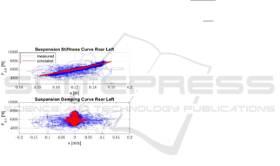
2.1.1 Suspension Model
From experimental data presented in section 4, it has
been proven that the stiffness curve of the suspen-
sion can be approached better using a non-linear rela-
tion. This allows the model to represent the physical
system better and will therefore further enhance esti-
mation performance. Additionally, less tuning of the
estimator noise matrices is required to acquire accu-
rate results. The stiffness curve can be expressed as a
function of the form:
F
z,k
= Ae
(B|r
r
r
sa
−r
r
r
wa
|)
(4)
where |r
r
r
sa
− r
r
r
wa
| is the distance from the suspension
attachment point to the wheel attachment point and A
and B are parameters defined to tune the curve. The
stiffness curve parameters were determined by fitting
the non-linear curve through experimental data using
a non-linear least squares method. The parameters
were set to A = 500 and B = 14 which leads to the
fitted data presented in the upper graph of figure 3.
Figure 3: The non-linear suspension stiffness (upper) and
linear suspension damping (lower) curve.
Next to this, a linear damping model is used with
the following characteristic equation:
F
z,c
= cv (5)
where c is the damping constant and v the velocity
of the suspension attachment point in the direction of
the suspension strut. Similar to the stiffness parame-
ters, the damping constant has also been tuned based
on experimental data and has been set to 5000 Ns/m.
The lower graph of figure 3 compares the simulated
versus the measured damping curve for this parame-
ter. The overall suspension force is then calculated
by summing the contributions from the stiffness and
damping curve:
F
z
= F
z,k
+ F
z,c
(6)
2.1.2 Tire Model
The tire model used in this paper is a linear tire model
using constant cornering stiffnesses. This choice was
made because for the tests discussed in this paper, the
vehicle did not enter the non-linear part of the tire
characteristic and therefore the extension towards a
non-linear tire model is not needed.
The calculation of the tire forces starts with the
derivation of the longitudinal slip and sideslip angle
for each tire. In this work, the formulas are based on
the brush model (Svendenius and Wittenmark, 2003)
but altered slightly to prevent singularities at low ve-
locities or wheel lock-up:
κ
i j
=
(
v
x,i j
−ω
i j
r
whl
|v
x,i j
|
if v
x,i j
≥ 1
v
x,i j
− ω
i j
r
whl
if v
x,i j
< 1
(7)
α
y,i j
=
(
v
y,i j
|v
x,i j
|
if v
x,i j
≥ 1
v
y,i j
if v
x,i j
< 1
(8)
where v
x,i j
is the longitudinal wheel velocity. Here,
the index i indicates front or rear and j indicates left or
right. Furthermore, v
y,i j
represents the lateral wheel
velocity, ω
i j
the wheel angular velocity and r
whl
is
the wheel radius.
Furthermore, the tire forces can be expressed us-
ing a linear tire model with constant cornering stiff-
nesses by the following equations for respectively the
longitudinal and lateral force:
F
x,i j
= C
x,i
κ
i j
(9)
F
y,i j
= C
y,i
α
y,i j
(10)
where the cornering stiffnesses C
x,i
and C
y,i
were ob-
tained experimentally using tire force transducers. In
these equations, κ
i j
represents the longitudinal slip
and α
y,i j
the sideslip angle of each wheel.
2.2 Measurement Equations
In this work, sensors are considered which are com-
monly mounted on commercial vehicles or sensors
which could potentially significantly improve esti-
mation performance. These sensors include body
accelerations, yaw rate, suspension stroke measure-
ments, longitudinal and lateral velocity, wheel speed
encoders and the GPS. The measurement vector for
these respective sensors can be expressed as:
y =

˙
v
v
v
cog
ω
z
|r
r
r
sus
| v
x
v
y
˙
ω
i j
x y

T
(11)
where |r
r
r
sus
| = |r
r
r
sa,i j
− r
r
r
wa,i j
| and r
r
r
sa,i j
is the loca-
tion of the suspension attachment point and r
r
r
wa,i j
is
the location of the wheel attachment point. All other
measurements are states of the estimator.
Design and Validation of a Multi-objective Automotive State Estimator for Unobservable and Non-linear Vehicle Models
275

2.3 Quantities of Interest
The quantities of interest need to be defined which
will be the targets of the estimator. Since this paper
presents an approach for multi-objective estimation,
multiple quantities of interest are defined. Therefore,
the following quantities of interest are targeted by the
estimator:
• Rear left wheel forces (F
x,rl
, F
y,rl
and F
z,rl
)
• Sideslip angle at body center of gravity (β)
• Vehicle trajectory (x, y)
The complete quantities of interest vector can thus be
expressed as:
y
y
y
vs
=

F
x,rl
F
y,rl
F
z,rl
β x y

(12)
=

F
x,rl
F
y,rl
F
z,rl
arctan

v
y
v
x

x y

(13)
where the tire forces F
x,rl
, F
y,rl
and F
z,rl
are calculated
as mentioned in (Vaseur et al., 2020) and x and y are
the position states of the estimator.
Tire forces and the sideslip angle are selected as
these variables are useful for advanced control algo-
rithms but not directly measurable in a cost-effective
manner. Additionally, the vehicle position is chosen
to showcase the benefits of the observability analysis
presented in section 3 on a real vehicle case as these
states are commonly unobservable in automotive esti-
mators.
2.4 Extended Kalman Filter
Application
In this work, the Extended Kalman Filter (EKF) is se-
lected as this filter is a straightforward extension of
the efficient linear Kalman filter for non-linear sys-
tems. Linearization, discretization and estimator set
up are performed according to the work in (Devos
et al., 2021). For this particular application, the dis-
cretized dynamic state-space equations form the ba-
sics of the estimation framework and can be expressed
using the linearized Jacobians as:
x
x
x
k+1
= F
F
F
k
x
x
x
k
+ B
B
B
k
u
u
u
k
(14)
y
y
y
k+1
= H
H
H
k
x
x
x
k+1
(15)
y
y
y
vs,k+1
= G
G
G
k
x
x
x
k+1
(16)
where F
F
F is the system Jacobian matrix, x
x
x is the state
vector, y
y
y is the measurement vector, H
H
H is the mea-
surement Jacobian, k is the timestep and B
B
B and u
u
u are
respectively the input Jacobian and the input vector.
Here, the linearized Jacobians F
F
F
k
, H
H
H
k
and G
G
G
k
are
saved every timestep for use during the observabil-
ity analysis as discussed in section 3. Finally, they are
used to calculate the EKF covariance equations and
state updates as documented in (Devos et al., 2021).
2.5 Sensor Selection
As a final point of attention, this work aims at se-
lecting the appropriate sensors for the estimation ap-
plication using the methodology presented in (Devos
et al., 2021). The methodology proposes to evalu-
ate the sensor performance before they are acquired
based on their relative contribution to the quantities
of interest covariance and has proven to deliver con-
sistent results for non-linear models.
3 OBSERVABILITY ANALYSIS
Observability is an important estimator property
which determines whether the targeted quantities of
interest can be estimated with a bounded uncertainty.
As this work features an EKF based framework, the
Jacobians are linearized every timestep and therefore
the result of linear observability tests can also change.
To analyze global observability, the total observability
matrix is used which combines observability matrices
calculated at evenly spaced timesteps and can be ex-
pressed as:
O
tot
=






O
1
O
1+p
O
1+2p
.
.
.
O
m






(17)
where the integer parameter p indicates how many ob-
servability matrices are taken into account.
3.1 Determining Unobservable States
Using the previously defined total observability ma-
trix, information can be extracted on which states are
unobservable. The first step is to calculate the kernel
of the total observability matrix:
V
V
V
u
= null(O
tot
) (18)
The resulting matrix V
V
V
u
contains the vectors which
span the null space of the observability matrix. If the
total observability matrix is full of rank, V
V
V
u
will not
contain any base vectors. However, if at least one
state is unobservable, V
V
V
u
will contain as many vec-
tors as unobservable states. Because the vectors of V
V
V
u
provide an orthogonal base to span the kernel of the
observability matrix, the entire matrix V
V
V
u
will have
near zero contributions except for the unobservable
states which makes it possible to identify them. One
possible algorithm is to check for non-zero contribu-
tions in the rows of the kernel vectors as described by
algorithm 1. Here, n is the number of states and x
x
x
u
are
VEHITS 2022 - 8th International Conference on Vehicle Technology and Intelligent Transport Systems
276

Algorithm 1: Unobservable state detection algorithm.
1: x
x
x
u
= [];
2: for i = 1 : n do
3: if mean(V
u
(i,:)) > threshold then
4: x
x
x
u
= [x
x
x
u
, i];
the unobservable states as detected by the algorithm.
The threshold value depends on the precision of the
machine and was set to 10
−10
for this work. For the
pseudo-code presented in algorithm 1, the assumption
has been made that the columns of the matrix V
V
V
u
con-
tain the kernel base vectors.
3.2 Dynamic Coupling Analysis using
the Linearized System Jacobian
When the unobservable states have been identified,
further analysis can be done on what causes these
states to be unobservable. As the observability ma-
trix is determined by the linearized sytem and mea-
surement Jacobians F
F
F
k
and H
H
H
k
, unobservable states
are the cause of both the lack of contributions in the
measurement Jacobian and the lack of dynamic cou-
pling between the vehicle states in the system Ja-
cobian. This dynamic coupling heavily determines
which measurements are needed to ensure full observ-
ability.
When the unobservable states have been deter-
mined, equations 14, 15 and 16 can be partitioned
such that the unobservable states are gathered in the
lower part of the state-space vector. The following
model equation is obtained:

˙
x
x
x
o
˙
x
x
x
u

k+1
=

F
F
F
oo
F
F
F
ou
F
F
F
uo
F
F
F
uu

k

x
x
x
o
x
x
x
u

k
+

B
B
B
o
B
B
B
u

k
u
u
u
k
(19)
where x
x
x
o
are the observable states and x
x
x
u
are the un-
observable states. From this equation, the following
cases can be derived:
F
F
F
ou
6= 0
0
0 & F
F
F
uo
6= 0
0
0: In this case, the model is highly
coupled and the system Jacobian is fully occu-
pied as depicted on the left matrix of figure 4.
Here, sensors which have contributions to only
a few states instantly cause all states to be theo-
retically observable due to the dynamic coupling
in the model. In practice however, the coupling
might be weak which can still lead to unobserv-
able states.
F
F
F
ou
= 0
0
0: In this case, the equations are partially de-
coupled and the system Jacobian is of the form as
presented by the middle matrix of figure 4. A typ-
ical example are systems containing friction mod-
els as the friction force usually depends on the
normal force but not vice versa.
F
F
F
ou
= 0
0
0 & F
F
F
uo
= 0
0
0: In this case, the equations are
decoupled and the system Jacobian is of the form
as presented by the right matrix of figure 4. For
this case, no dynamic coupling exists between the
states x
x
x
o
and x
x
x
u
in the model.
Figure 4: Different possible layouts of the system Jacobian
matrix F
F
F
k
.
In this work, the vehicle model can be categorized
by the second case where F
F
F
ou
= 0
0
0. The partially de-
coupled state vector x
x
x
u
consists of the vehicle longi-
tudinal and lateral position. Because these states are
partially decoupled, they will be unobservable if their
corresponding measurements are not taken into ac-
count due to the lack of dynamic coupling. This leads
to stability issues as the covariances of these states
will be unbounded. In case these unobservable states
do not depend on the quantities of interest, an observ-
able transformation can be deployed to stabilize the
unobservable covariances. The transformation can be
expressed as:
x
x
x = V
V
V
T
o
q
q
q (20)
where V
V
V
o
is the observable part of the mode ma-
trix V
V
V resulting from a Singular Value Decomposition
(SVD) of the total observability matrix O
tot
.
A final point of attention is that, even though the
system Jacobian could be fully coupled, it might still
occur that the observability matrix is ill-conditioned if
the values inside the Jacobian matrix are very small.
A weak coupling is then present between the states
which means that they theoretically depend on each
other, but in practice the coupling is so small that they
can be unobservable.
4 EXPERIMENTAL RESULTS
The proposed estimator approach has been validated
on an electric vehicle case namely the Range Rover
Evoque shown on Figure 5. The data was gener-
ated during a test campaign at Ford Lommel Proving
Ground by (Van Aalst et al., 2018) and (Vaseur et al.,
2020) and graciously provided to us for validation of
this work. The vehicle was equipped with an SBG
Inertial Measurement Unit (IMU) to measure acceler-
ations, velocities, positions and angles, a Corrsys Da-
tron optical sensor to obtain the sideslip angle, sus-
Design and Validation of a Multi-objective Automotive State Estimator for Unobservable and Non-linear Vehicle Models
277

pension stroke measurements and Kistler tire force
transducers. The vehicle CAN bus was also logged
to measure the inputs to the model namely the steer-
ing wheel angle, motor torques and brake torques. All
relevant vehicle parameters used to evaluate the equa-
tions are defined in table 1.
Figure 5: The Range Rover Evoque used on test track 7 at
Ford Lommel Proving Ground (Van Aalst et al., 2018).
Table 1: Vehicle model parameters for the Range Rover
Evoque (Naets et al., 2017).
Vehicle Property Abbr Value
Vehicle mass m 2408kg
Roll moment of inertia I
x
615kgm
2
Pitch moment of inertia I
y
1546kgm
2
Yaw moment of inertia I
z
3231kgm
2
Distance COG - front axle l
f
1.439m
Distance COG - rear axle l
r
1.236m
Track width front t
f
1.625m
Track width rear t
r
1.625m
Height of COG h
COG
0.65m
Front cornering stiffness C
y f
88.500N/rad
Rear cornering stiffness C
yr
118.200N/rad
Wheel radius r
whl
0.3597m
Wheel inertia I
whl
4kgm
2
4.1 Covariance Tuning
In this work, the estimator has been tuned by trial-
and-error. The following (constant) values were used
to populate the noise matrix Q
Q
Q
d
:
Q
v
x
,v
y
,v
z
= 1 · 10
−4
,Q
˙
φ,
˙
θ,
˙
ψ
= 1 · 10
−3
Q
x,y,z
= 1 · 10
−5
,Q
φ,θ,ψ
= 1 · 10
−1
,Q
ω
i j
= 1 · 10
−5
where Q
v
x
,v
y
,v
z
represents the translational velocity
noise, Q
˙
φ,
˙
θ,
˙
ψ
the rotational velocities noise, Q
x,y,z
the
position noise, Q
φ,θ,ψ
the angular noise and Q
ω
i j
the
wheel angular velocity noise.
Subsequently, the measurement noise was derived
from specification sheets and tests executed in previ-
ous work by (Van Aalst et al., 2018) and were defined
as:
R
a
i
= 3.1 · 10
−3
(m/s
2
)
2
,R
gyr
= 2.5 · 10
−1
(m/s)
2
R
GPS
= 2m
2
,R
ω
i j
= 2.1 · 10
−1
(m/s)
2
where R
a
i
is the MEMS accelerometer noise of the
IMU, R
gyr
the gyroscope noise of the IMU, R
GPS
the
GPS noise, R
ω
i j
the wheel speed encoder noise.
4.2 Results and Discussion
The results of this work are clustered in three main
sections as elaborated upon in this paper. To start,
the appropriat sensors were selected according to the
methodology presented in subsection 2.5. Subse-
quently, the synchronization capabilities are shown
together with the limitations for unobservable, decou-
pled states as discussed in section 3. Finally, the esti-
mator multi-objective performance is discussed show-
ing the results for the targeted quantities of interest.
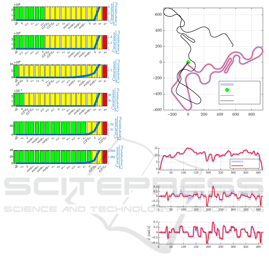
4.2.1 Sensor Selection
Figure 6 shows the results of the sensor selection al-
gorithm where the blue line indicates the rise in co-
variance when the sensor is removed from the esti-
mator. The bar colors indicate whether observability
is fulfilled (green), partially fulfilled but can be stabi-
lized by the projection defined in section 3.2 (yellow)
or not fulfilled (red).
The figure confirms that some sensors indeed have
significant contributions to multiple quantities of in-
terest. Accelerations for example are important when
estimating tire forces as they are directly related to the
forces in the equations of motion. Additionally, figure
6 also shows that for the planar tire forces (F
x
and F
y
),
the yaw rate (
˙
ψ) is an important sensor whereas for
the vertical tire force, the suspension stroke measure-
ments are more important. On the other hand, GPS
measurements are less relevant for the tire forces but
are required when the vehicle trajectory states are part
of the targeted quantities of interest. As indicated
by the yellow and red bar colors, position states are
automatically unobservable when GPS measurements
are omitted due to their decoupled nature. All of the
conclusions based on the results presented in figure 6
stroke with engineering experiences.
To ensure a good tracking of all the quantities of
interest as defined in subsection 2.3, the results pre-
sented in figure 6 together with availability on com-
mercial vehicles and cost were used to select the sen-
sors for this estimator. In the end, the following sen-
sors were chosen:
• Body accelerations (a
x
, a
y
and a
z
)
• Yaw rate (
˙
ψ)
• Wheel speed encoders (ω
i j
)
• GPS (x, y)
4.2.2 Synchronization Capabilities and
Observability Analysis
When the vehicle trajectory states are part of the es-
timator quantities of interest, GPS measurements are
VEHITS 2022 - 8th International Conference on Vehicle Technology and Intelligent Transport Systems
278

Longitudinal tire force rear left
Covariance
Lateral tire force rear left
Covariance
Vertical tire force rear left
Covariance
Sideslip angle
Covariance
Vehicle position East
Covariance
Vehicle position North
Covariance
Figure 6: Results of the sensor selection ranking procedure.
The x-axis represents cumulative removed sensors from the
sensor space. The color of the bars indicate observability
(green is observable, yellow is unobservable but stable and
red is unobservable and unstable). The blue line visualizes
the normalized covariance rise when omitting sensors.
important to deliver interpretable results. This is be-
cause these states are partially decoupled from the
other ones as discussed in section 3 and therefore re-
quire GPS measurements to be observable. Figure 6
confirms this because, for every quantity of interest,
as soon as the GPS measurement in either x or y di-
rection is omitted, the yellow bar indicates that the
estimator is unobservable but can be stabilized using
the transformation defined in equation 20. Figure 7
shows that for unobservable position states, the vehi-
cle trajectory is not correctly tracked even when ap-
plying the observable transformation of equation 20
which stabilizes the position covariances. Therefore,
unobservable states and their associated covariances
cannot be reliably interpreted and should be handled
with care.
Figure 8 compares the simulated vehicle velocities
and yaw rate versus measurements. These variables
show that the estimator can synchronize the model
well with the measurements using previously selected
sensors. Additionally, these variables are currently
widely used in ESP systems of commercial vehicles
East [m]
North [m]
Vehicle trajectory and GPS measurement
GPS
start/stop
observable
unobservable
Figure 7: Simulated versus GPS measured trajectory for
both an unobservable and observable simulation.
Time [s]
v [m/s]
Vehicle Longitudinal velocity
measured
simulated
Time [s]
v [m/s]
Vehicle Lateral velocity
Time [s]
Vehicle Yaw Rate
Figure 8: Estimation results versus measurements for the
validation case: planar velocities and yaw rate.
and could therefore also be targeted by the estimator
for use in advanced control algorithms.
4.2.3 Multi-objective Estimation
The resulting tire forces and vehicle sideslip angle can
be seen in figure 9. The figure shows that the es-
timator is capable of determining the tire forces as
well as the vehicle sideslip angle although the lat-
eral tire forces are slightly over-estimated compared
to the measurements. A possible explanation is that
the road is assumed flat as including road angles is
not a straightforward task. Nevertheless, the estimator
shows reliable results for the targeted quantities of in-
terest. When comparing to similar results for single-
Design and Validation of a Multi-objective Automotive State Estimator for Unobservable and Non-linear Vehicle Models
279

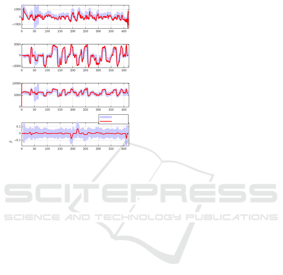
Time [s]
F
x,rl
[N]
Rear Left Longitudinal Tire Force
Time [s]
F
y,rl
[N]
Rear Left Lateral Tire Force
Time [s]
F
z,rl
[N]
Rear Left Vertical Tire Force
Time [s]
COG
[rad]
Vehicle Sideslip Angle
measured
simulated
Figure 9: Estimation results for the rear left wheel forces
and the vehicle sideslip angle.
objective estimators, one can observe that the sensors
used for both tire force and sideslip angle estimation
are mostly identical which is confirmed by the sensor
selection results on figure 6. This approach is able to
combine both quantities of interest in a single estima-
tor and additionally provides improved performance
due to the coupled dynamic nature of the model.
5 CONCLUSIONS
In this work, a novel, multi-objective, automotive
state estimator has been developed featuring a system-
level, non-linear vehicle model. As estimators us-
ing more complex models typically face more issues
towards stability, an extensive observability analysis
was performed. It is shown that unobservable states
can be detected using a Singular Value Decomposi-
tion of the total observability matrix and that dynamic
model coupling greatly determines the required sen-
sors to obtain an observable estimator. Using an ob-
servable projection defined in previous work, this pa-
per proves that it is possible to stabilize the estimator
without GPS measurements if they are independent
from the quantities of interest due to their decoupled
nature. Finally, the estimator has been experimentally
validated on an engineering vehicle case and proved
to be able to accurately track all quantities of interest
with a minimal sensor set.
ACKNOWLEDGEMENTS
This research was partially supported by Flanders
Make, the strategic research centre for the manu-
facturing industry. The Flanders Innovation & En-
trepreneurship Agency within the IMPROVED and
MULTISENSOR project is also gratefully acknowl-
edged for its support. Internal Funds KU Leuven are
gratefully acknowledged for their support.
REFERENCES
Albinsson, A., Bruzelius, F., Jonasson, M., and Jacobson,
B. (2014). Tire force estimation utilizing wheel torque
measurements and validation in simulations and ex-
periments. In 12th International Symposium on Ad-
vanced Vehicle Control, pages 294–299.
Devos, T., Kirchner, M., Croes, J., Desmet, W., and Naets,
F. (2021). Sensor selection and state estimation for
unobservable and non-linear system models. Sensors,
21(22).
Kim, D., Min, K., Kim, H., and Huh, K. (2020). Vehicle
sideslip angle estimation using deep ensemble-based
adaptive kalman filter. Mechanical Systems and Signal
Processing, 144:106862.
Naets, F., van Aalst, S., Boulkroune, B., Ghouti, N. E., and
Desmet, W. (2017). Design and experimental vali-
dation of a stable two-stage estimator for automotive
sideslip angle and tire parameters. IEEE Transactions
on Vehicular Technology, 66(11):9727–9742.
Nakamura, W., Hashimoto, T., and Chen, L.-K. (2020).
State estimation method based on unscented kalman
filter for vehicle nonlinear dynamics. International
Journal of Electrical and Information Engineering,
14(12):435 – 438.
Reif, K., Renner, K., and Saeger, M. (2007). Vehicle
state estimation on the basis of a non-linear two-track
model. ATZ worldwide, 109:33–36.
Svendenius, J. and Wittenmark, B. (2003). Brush tire model
with increased flexibility. In European Control Con-
ference, pages 108–115.
Van Aalst, S., Naets., F., Boulkroune, B., De Nijs, W., and
Desmet, W. (2018). An adaptive vehicle sideslip es-
timator for reliable estimation in low and high excita-
tion driving. In 15th IFAC Symposium on Control in
Transportation Systems, volume 51, pages 243–248.
Vaseur, C., van Aalst, S., and Desmet, W. (2020). Vehicle
state and tire force estimation: Performance analysis
of pre and post sensor additions. In 2020 IEEE Intel-
ligent Vehicles Symposium (IV), pages 1615–1620.
Wang, R. and Wang, J. (2013). Tire–road friction coeffi-
cient and tire cornering stiffness estimation based on
longitudinal tire force difference generation. Control
Engineering Practice, 21(1):65–75.
Yang, C., Blasch, E., and Douville, P. (2010). Design of
schmidt-kalman filter for target tracking with naviga-
tion errors. In IEEE Aerospace Conference Proceed-
ings, pages 1–12.
VEHITS 2022 - 8th International Conference on Vehicle Technology and Intelligent Transport Systems
280