Analysis of Coastline Evolution using Landsat and Sentinel 2 Images

from 2001 to 2020 in Callao Bay, Peru

Amanda Muñoz

, Luis Mendoza

, Emanuel Guzmán

and Carmela Ramos

Facultad y Escuela de Ingeniería Civil, Universidad Peruana de Ciencias Aplicadas,

Av. Prolongación Primavera 2390, Santiago de Surco, Lima, Peru

Keywords: Coastal Erosion, Coastal Accretion, Satellite Images, Callao Bay.

Abstract: The study presented an analysis of the shoreline evolution in Callao Bay – Lima, Perú; which is one of the

most important bays in Perú due to economics and touristic activities. Study areas include La Punta, Callao

and Ventanilla districts with an approximate 32 km of length. The study area was divided into six sectors, and

the analysis was focused mainly from the 2001 to 2020 period, identifying areas affected by coastal erosion

or accretion throughout. Satellite data images were obtained from Landsat (5, 7 and 8) and Sentinel 2, they

were processed to correctly identify the shoreline. Shoreline variations were analyzed using the DSAS (Digital

Shoreline Analysis System) utility, applying a statistical method called "Linear Regression Ratio". Shoreline

variations showed different rates of changes along different sectors of the study area. In general terms, the

accretion or erosion trend in Callao Bay was a low accretion with average rates from 3.77 m / year to 4.20 m

/ year, except in the sector which is closed to the Rímac river with change rate of around 11.85 m/year.

1 INTRODUCTION

The constant growth of the population, the flow of

economic activities and mismanagement of water use,

have directly affected the deterioration of the water

resources (Sánchez, 2019). This is directly related to

the shoreline, which is of vital importance for the

improvement of social, economic, and recreational

opportunities; in other words, it is fundamental for the

development of the economic and natural

environment (Yasir et al., 2020). However, the

hazards affecting the coastal zone have increased over

the years, resulting from rapid changes in various

physical and geological variables that have been

influenced by dynamic coastal processes. Likewise,

the coastal zone and the water quality has undergone

changes due to the influences of anthropogenic

activities such as piers and beach protection structures

(Sheik Mujabar & Chandrasekar, 2013). This

problem is mentioned in a study by Soto (2018),

where he highlights how the northern and central

coast of Perú has been affected by sediments

generated by marine currents and the erosion of river

https://orcid.org/0000-0002-3512-587X

https://orcid.org/0000-0001-7890-9597

https://orcid.org/0000-0001-8381-4509

https://orcid.org/0000-0002-4269-2944

basins such as the Rímac and Chillón (Soto, 2018). In

addition, the metropolitan area of Lima has been

affected by constant changes in the shoreline of the

Callao Bay (Guzman et al., 2020); specifically in the

area near the Callao Port Terminal with a rate of

3m/year between the years 1984 to 2016 (Luijendijk

et al., 2018). On the other hand, El Niño, an extreme

factor, has a great influence on the displacement of

the shoreline in Callao Bay (Guzman et al., 2020).

Therefore, the study of the constant change of the

coastline is important so that, based on this, a water

resource management strategy can be developed and

the negative effects, such as chemical and dynamic

imbalance of the coast, loss of coastal biodiversity,

and decrease in gross national product (GDP), can be

avoided (Rangel-Buitrago et al., 2015). Satellite

imagery has been used, to monitor changes along the

coastal zone, because it provides repeatable and

consistent statistics of variations. In addition, the

combination of this methodology with Geographic

Information System (GIS) for monitoring the

evolution of coastlines on a temporal scale, presents

Muñoz, A., Mendoza, L., Guzmán, E. and Ramos, C.

Analysis of Coastline Evolution using Landsat and Sentinel 2 Images from 2001 to 2020 in Callao Bay, Peru.

DOI: 10.5220/0011037500003185

In Proceedings of the 8th International Conference on Geographical Information Systems Theory, Applications and Management (GISTAM 2022), pages 115-122

ISBN: 978-989-758-571-5; ISSN: 2184-500X

115

a digital structure that facilitates the detection of

vulnerable areas (Yasir et al., 2020).

The present study includes the use of Landsat (5,7

and 8) and Sentinel 2 satellite images, to visually

identify land and water coverage, also manually

obtaining the annual shorelines variations from 2001

to 2020. An analysis of the accretion or erosion

tendency of the shoreline will be present through the

application of Digital Shoreline Analysis System

(DSAS) which is a tool that allows statistical methods

such as Linear Regression Ratio (LRR) to be applied

to a set of annual coastlines to determine their

movement and trends.

2 METHODOLOGY

2.1 Study Area

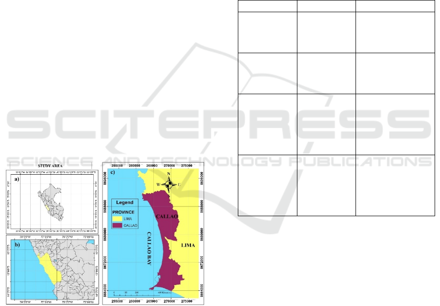
Callao Bay is located on the central coast of Perú and

belongs to the department of Lima and the Callao

Constitutional Province (Figure 1); it also covers La

Punta, Callao and Ventanilla districts. Callao Bay is

one of the most important bays in Perú due to

economics activities that are developed (Callao Port,

fishing industry, touristic activities such fishing and

water sport). One of the special characteristics of the

study area is the presence of the Chillon and Rimac

Rivers mouths and Callao port installations.

Figure 1: a) Peru, b) Lima and c) Districts covered by the

study area.

2.2 Data Sources

Images from Landsat and Sentinel 2 satellites were

used for the development of the study since they

facilitate the remote sensing of the characteristics in

the area to be studied. Both satellite image sources are

freely available and were obtained from the US

Geological Survey’s (USGS) Earth explorer website

(http://earthexplorer.usgs.gov)

To analyze shoreline variations in study area, one

satellite image per year was selected, taking into

consideration that an annual coastline was required,

and the area shows a constant low tide height with an

average of 54 cm per month that was maintained even

during the 2017 El Niño phenomenon

(DIHIDRONAV, 2020)

The area shows a lot of cloud cover, which made

its identification difficult. Therefore, the resolution of

the band sets belonging to each satellite were

important characteristics to take into consideration

(Table 1).

Table 1: Annual satellite image and resolution.

SATELLITE YEARS RESOLUTION

Landsat 7

2001, 2002,

2003, 2004,

2012, 2013,

2014 and 2015

Bands 1 to 7

(30 m/pixel)

Bands 8

(

15 m/

ixel

)

Landsat 5

2005, 2006,

2007, 2008,

2009, 2010

and 2011

Bands 1 to 7

(30 m/pixel)

Landsat 8 2020

Bands 1 to 7 and 9

(30 m/pixel)

Bands 8

(15 m/pixel)

Bands 10 and 11

(100 m/pixel)

Sentinel 2

2016, 2017,

2018 and 2019

Bands 1, 9 and 10

(60 m/pixel)

Bands 2 to 4 and 8

(10 m/pixel)

Bands 5 to 7, 8, 11

and 12 (20 m/pixel)

Therefore Table 2 shows the satellite images, the day

they were taken, along with the name and bands that

were used.

2.3 Image Pre-Processing and

Coastline Detection

For this research work, pre-processing steps were

applied, using the "Semi-Automatic Classification"

plugin of the QGIS program, which simplified the

manual extraction of the shoreline.

GISTAM 2022 - 8th International Conference on Geographical Information Systems Theory, Applications and Management

116

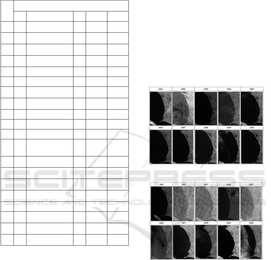
Table 2: Characteristics of the satellite images used.

YEAR

CHARACTERISTICS OF THE SATELLITE IMAGES

USED (2001-2020)

SAT. NAME DAY

START

TIME

BANDS

2001 L7

LT05_L1TP_007068_200

11122_20161209_01_T1

11/22 14:50:15

4, 5, 6

and 7

2002 L7

LE07_L1TP_008068_200

21226_20170127_01_T1

12/26 15:05:15

1, 2, 3, 4,

5,6 and 7

2003 L7

LE07_L1TP_008068_200

30401_20170125_01_T1

04/01 15:05:38

4,5,6,7,

and 8

2004 L7

LE07_L1TP_007068_200

40123_20170123_01_T1

01/23 14:59:45

3,4,5,6,7

and 8

2005 L5

LT05_L1TP_008068_200

50430

20161126

04/30 15:04:07 5 and 7

2006 L5

LT05_L1TP_008068_200

60503

20161122

04/03 15:08:52 5

2007 L5

LT05_L1TP_007068_2007

0328_20161116_01_T1_d

03/28 15:05:50

1, 4, 5

and 7

2008 L5

LT05_L1TP_008068_200

80321_20161101_01_T1

03/21 15:06:48

2, 3, 4, 5

and 7

2009 L5

LT05_L1TP_008068_200

90425

20161026

04/25 15:04:18 5 and 7

2010 L5

LT05_L1TP_008068_201

00514

20161015

05/14 15:07:42 4, 5 and 7

2011 L5

LT05_L1TP_007068_201

10307

20200823

03/7 15:00:40 5, 6 and 7

2012 L7

LE07_L1TP_008068_201

20104_20200909_02_T1

01/04 15:10:56

1, 2, 3,

4,5,6,7

and 8

2013 L7

LE07_L1TP_007068_201

30405_20200907_02_T1

04/05 15:06:47

1, 6, 7

and 8

2014 L7

LE07_L1TP_008068_201

40125_20200906_02_T1

01/25 15:13:41

2, 3, 4, 5,

6 and 7

2015 L7

LE07_L1TP_008068_201

50317_20200905_02_T1

03/17 15:15:54

5, 6, 7

and 8

2016 S2

L1C_T18LTM_A007887_

20161225T152814

12/25 15:28:14

2, 3,4, 8,

11 and 12

2017 S2

L1C_T18LTM_A008416_

20170131T152508

01/31 15:25:08 2 and 3

2018 S2

L1C_T18LTM_A004584_

20180121T151656

01/21 15:16:56

2, 3, 4

and 8

2019 S2

L1C_T18LTM_A018855_

20190131T152414

01/31 15:24:14

2, 3, 4

and 8

2020 L8

LC08_L1TP_007068_202

01126_20210316_02_T1

11/26 15:11:02

1, 2, 6

and 7

2.3.1 Image Pre-processing using QGIS

With the QGIS version 3 plugin, the preprocessing

was performed to achieve the highest sharpness of the

study area comprising the satellite images for the

separation of water and land covers from the annual

images.

A clip was created for all the bands and the

respective atmospheric corrections using the

DarkObject Subtraction 1 (DOS1) method (Luca

Congedo, 2016), to achieve a complete visualization

without noise (visual obstacles in the raster).

Subsequently, the combination of bands was

performed with different resolutions such as

10m/pixel for Sentinel 2 ,15 m/pixel for Landsat 7

and Landsat 8, and 30m/pixel for Landsat 5. This to

achieve a sharper raster that allowed the identification

of the contrast between land and water.

On the other hand, for the years 2004, 2012, 2013

and 2015 only the Landsat 7 satellite image was

available, which since 2002 had a banding error due

to sensor failure. However, a reliability analysis using

a percentage fraction of the parts that are not visible,

due to the band error, with the total length of the zone.

Led to the conclusion that this failure would not

significantly affect the visual identification of the

coastline. Figure 2 shows the corrected satellite

images for the years between 2001 and 2010 and

Figure 3 shows the corrected satellite images for the

years between 2011 and 2020.

Figure 2: Processed satellite images for years 2001 to 2010.

Figure 3: Processed satellite images for years 2011 to 2020.

2.3.2 Shoreline Detection

The detection of the shoreline, belonging to the

Callao Bay, was performed manually, and validated

by importing the polyline into Google Earth where it

was georeferenced by date and UTM coordinates.

The difference in the range of colors, presented by the

satellite images (raster), was considered and in this

way the limit between the white pixels (land covers)

and black pixels (sea covers) was determined. In

addition, the creation of the polyline for the coastline

representation was performed with the multiline tool

and in the most precise way to avoid taking non-

Analysis of Coastline Evolution using Landsat and Sentinel 2 Images from 2001 to 2020 in Callao Bay, Peru

117

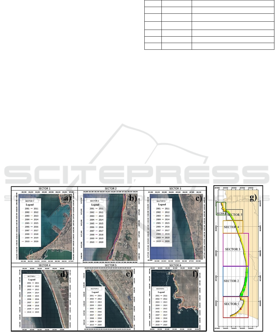
coastal structures. To perform the analysis, study area

was divided into 6 sectors (Figure 4).

The creation of these sectors was made

considering the extension of the shoreline; as well as

the presence of structures such as the Perú Port

Terminal and natural elements such as the mouths of

the Rímac and Chillón rivers (Table 3).

2.4 DSAS Applications

After collecting the coastlines, belonging to the

period 2001 to 2020, with QGIS these were exported

in “shape” format to ArcGIS 10.5 and the “Merge”

tool was applied to create a single image that would

comply all the polylines (20 shorelines). Then, the

“Buffer” tool was applied to the compilation of lines

to obtain an equidistant margin at 150 meters.

Afterwards, geographic database file was created,

where two parameters were added for analysis; with

names of Coastal Lines and Baseline and were

georeferenced in the UTM WGS84 18S zone.

The “Digital Shoreline Analysis System” (DSAS)

was used for the analysis of the evolution in the

shoreline. Then, the transects were designed with a

spacing of 20 meters and a maximum distance from

the baseline of 500 meters, considering the sinuosity

of the terrain.

Table 3: Mainly characteristics of sectors analysis in study

area.

Secto

Length (km) Observations

1 6.95 Presence of the Perú Port Terminal

2 7.18 Rímac mouth is located

3 8.44 Chillón mouth is located

4 3.49 Start zone of Ventanilla’s wetlands

5 2.72 End zone of Ventanilla’s wetlands

6 3.32 Presence of littoral cliffs

Finally, once the transects were obtained, the data

of the intersections between the shorelines and the

transects were extracted.

The specified distances indicate how many meters

there are between the shorelines of the period and the

baseline that was previously created equidistant from

the union of the shorelines.

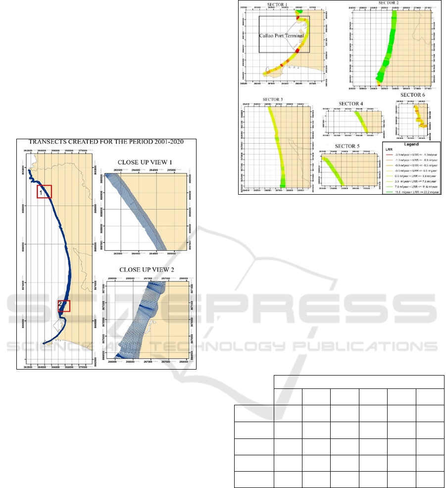
In Figure 5 a map with the transects generated for

the shorelines by year and belonging to the period

2001-2020. In this regard, it is important to mention

that, although for greater precision the intersection of

the transects should be avoided, due to the concave or

sinuous shape of the bay, the intersection of the

transects could not be totally reduced. However, the

few areas where these intersections exist, the close up

view 2 of Figure 5, would not be generating a great

impact on the analysis for the proposed study.

Figure 4: Shorelines from 2001 to 2020 for each sector, a) Sector 1, b) Sector 2, c) Sector 3, d) Sector 4, e) Sector 5, f) Sector

6 and g) Sector Overview.

GISTAM 2022 - 8th International Conference on Geographical Information Systems Theory, Applications and Management

118

2.5 Statistical Analysis of Shoreline

Change Rates

After obtaining the transects, a statistical analysis was

performed using LRR method; since one of the

advantages of this method is that it considers all the

shorelines, thus giving a more detailed analysis (Yasir

et al., 2020). For this reason, the DSAS “Calculation

of ratios” tool was used, where the rates of change of

the shoreline were calculated throughout the 20-year

period with the LRR method.

Figure 5: Transects created from the shorelines from 2001

to 2020. In approach 2 it was observed that intersections of

the transects that were created due to the sinuousness of the

land were created; however, its presence did not

significantly affect the calculations performed. Then rates

obtained by the LRR method represented with color gamut.

In Figure 6 the different trends for each sector are

shown. Likewise, the transects (132 to transect 317)

that belonged to the “Terminal Portuario del Perú”

were identified, since these transects would not enter

the statistical analysis.

To perform the analysis of the variation of the

shoreline, the distance data between the shorelines

and the baseline extracted from each transect,

manually taking 100% of the rates. A subtraction was

performed between the total distances of the

consecutive years, to then average the data and obtain

trends for each sector created.

Figure 6: LRR method in the sectorization of the Bay of

Callao and detail of sectors.

3 RESULTS

Table 4 shows a summary of the average rates of

sedimentation, erosion, maximum and minimum,

taking 95% of the significant rates. It was identified

that some sectors did not show negative erosion data;

however, rate trends have been declining over the

years.

Table 4: Table of average annual rates by sector applying

the DSAS tool (2001-2020).

From 2001 to 2020

Sector

Accretion

(m/year)

1.53 11.89 2.00 2.47 5.83 0.95

Erosion

(

ear

)

-1.06 -0.24 -0.44 DP DP -0.54

Maximum

(

ear

)

3.93 22.15 6.19 3.93 7.56 7.18

Minimum

(

ear

)

-3.85 -0.24 -1.57 0.23 3.62 -2.14

Average

(

ear

)

0.13 11.85 1.96 2.47 5.83 0.38

Note: DP means "Don't present"

In the same way, a graph was made (Figure 8) of the

average historical displacement of the shoreline from

2001 to 2020, which were scaled to achieve a global

visualization of the changes per year that have

suffered shoreline. Results are described as follows:

 It was observed that sector 1 remains stable,

having negative and positive rates of lower value.

It was also identified that most of the structures,

including springs and the Perú Port Terminal, are

in the sector, with a high anthropogenic influence.

Analysis of Coastline Evolution using Landsat and Sentinel 2 Images from 2001 to 2020 in Callao Bay, Peru

119

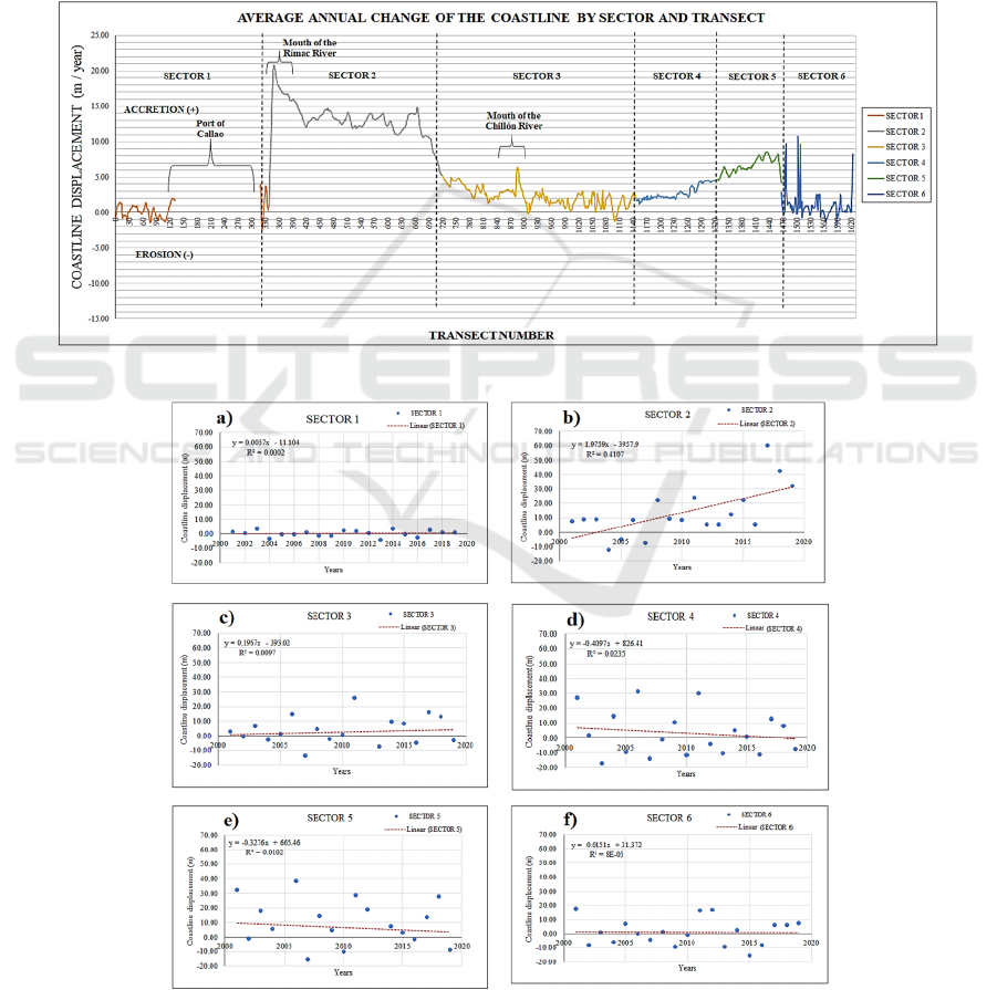
 In sectors 2, 4 and 5, an abrupt change was

identified that shows high sedimentation between

2016 and 2017, in which the El Niño phenomenon

occurred, generating great changes in the natural

factors that are present on the coast.

 Sector 3 has shown erosion and sedimentation

rates that have increased over the years, with a

global tendency to sediment slightly.

 Finally, sector 6, where it is noteworthy to

mention, has a large presence of cliffs, showed

higher moderate erosion rates, maintaining this

trend throughout the 20-year period.

In Figure 7 the displacement of the shoreline in m /

year is presented, where the positive value represents

sedimentation and the negative value represents

erosion, according to the transect number. The

highest peak occurs in the sector 2 (transect 349),

with a value of 22.15 m / year which is in the northern

area of the outlet of the Rímac River and the

maximum erosion occurs in sector 1 (transect 322),

with a value of -3.85 m / year located in the southern

part of the mouth of the Rímac River.

Figure 7: Transects created from shorelines from 2001 to 2020.

Figure 8: a) Historical analysis by LRR of sector 1, b) Historical analysis by LRR of sector 2, c) Historical analysis by LRR of

sector 3, d) Historical analysis by LRR of sector 4, e) Historical analysis by LRR of sector 5, f) Historical analysis by LRR of

sector 6.

GISTAM 2022 - 8th International Conference on Geographical Information Systems Theory, Applications and Management

120

4 DISCUSSIONS

After a comparison with the background of the study

presented, it was observed that the tendencies to

sediment or erode in some places along the coast of

Callao Bay have been maintained despite the

presence of extreme factors such as the El Niño

phenomenon. As mentioned by Teves and San

Román (2012) study, the area between the mouths of

the Rímac and Chillón rivers (Sector 2 and Sector 3)

has a large presence of sediments that are transported

towards the northern part of the mouths due to marine

currents (Teves & San Román, 2012). Similarly, the

creation of the trend map of the present study showed

this accretion between the mouths and the beaches

north to the area of the beginning of the cliffs, with a

notable increase for the year 2017; however, for

subsequent years, sedimentation rates were

decreasing minimally.

On the other hand, erosion is a very recurrent

process in the surroundings of “Mirador Playa

Pachacutec” in sector 6 (Figure 4), this largely due to

the steep slopes that occur in the place (Teves & San

Román, 2012). The trend map (Figure 8) created

shows high erosion rates that are decreasing until

showing slight sedimentation rates in certain parts of

the sector 6.

In addition, the R

factor obtained from the

historical analysis (Figure 8), shows a trend to present

accretion as it gets closer to 1 and the data present a

constant increase, otherwise, while the annual data

shows more negative points of erosion, the factor is

almost 0.

Likewise, the results obtained from this study

have the same sedimentation and coastal erosion

trends as Luijendijk's Aquamonitor interface. In this

study, the author analyzed the trends of coastlines

along the world's continents, showing very general

rates of coastal dynamics that could be taken as a base

for the present study. (Luijendijk et al., 2018). The

comparisons at the total average level are:

 This study shows a sedimentation rate of

0.13m/yr, 11.85m/yr, 1.96m/yr, 2.47m/yr,

5.83m/yr and 0.38m/yr with a difference with the

Aquamonitor of 0.26m/yr, 4.50m/yr, 0.37m/yr, -

3.31m/yr, -3.09m/yr and -1.00m/yr for sectors 1,

2,3,4,5 and 6 respectively.

 On the one hand, it is worth mentioning that the

Aquamonitor presents data from 1984 to 2016 and

is a global level study. On the other hand, our

study presents data from 2001 to 2020. The

differences in rates in sector 2 are mainly due to

the occurrence of the 2017 El Niño phenomenon

because there was a sediment peak of 60 meters.

5 CONCLUSIONS

From the analysis of the sectorization and in general

lines of the Callao Bay, it was observed that the trend

of the coastline is to present a slight sedimentation

with average rates between 3.77 to 4.2 m/year. In

addition, sector 2; showed a moderate and constant

trend throughout the period that, for the year 2017

suffered an accumulation of sediment that reached up

to 60 meters offshore. This is due to the presence of

the extreme phenomenon called El Niño, which

generated an accumulation of sediment on the

beaches located north of the mouths of the Rímac and

Chillón rivers.

The temporal analysis shows that sector 1, which

includes the Perú Port Terminal, has remained

constant when compared to the other sectors. The

rates for the 20-year period have had a minimal but

progressive increase. Likewise, sectors 2 and 5 have

high average sedimentation rates, which have been

decreasing in lower values for the last 3 years, since

the El Niño phenomenon.

Sector 6 presents high and constant erosion

values, due mostly to the presence of cliffs and high

slopes in the area; however, the average rate of the

sector is to present a slight sedimentation because a

large percentage of the rates are positive (Figure 7).

As mentioned above, a Linear Regression Ratio

statistical analysis was performed, which was

obtained manually and with the application of the

DSAS extension. It was observed that both methods

show similar trends in the long term. On the one hand,

the manual calculation allows to see the annual

evolution of changes in average rates, while the

DSAS shows an average rate for the 20-year period.

In other words, the extension applies statistical

methods and takes into consideration the shoreline

variations in each confidence interval.

Although the study manages to present erosion or

accretion trends for the study area, there is an error

range of 5 to 30 meters due to the different resolutions

of the satellites used. This affects manual shoreline

detection and subsequent statistical analysis.

Therefore, the use of higher resolution satellite

images or digital elevation models will allow an

automatic extraction of the shoreline and,

consequently, will improve the extracted data with a

smaller error interval than the one presented by the

study.

Analysis of Coastline Evolution using Landsat and Sentinel 2 Images from 2001 to 2020 in Callao Bay, Peru

121

REFERENCES

Congedo, L. Semi-Automatic Classification Plugin

Documentation (Release 6.0. 1.1). 2016.

DIHIDRONAV. (2020). Tabla de mareas. Retrieved from

https://www.dhn.mil.pe/portal/tabla-mareas#.

Guzman, E., Ramos, C., & Dastgheib, A. (2020). Influence

of the el nino phenomenon on shoreline evolution.

Case study: Callao bay, Peru. Journal of Marine

Science and Engineering, 8(2). https://doi.org/

10.3390/jmse8020090

Himmelstoss, E. A., Henderson, R. E., Kratzmann, M. G.,

& Farris, A. S. (2018). Digital Shoreline Analysis

System (DSAS) Version 5.0 User Guide. Open-File

Report 2018-1179, 126.

Luijendijk, A., Hagenaars, G., Ranasinghe, R., Baart, F.,

Donchyts, G., & Aarninkhof, S. (2018). The State of

the World’s Beaches. Scientific Reports, 8(1), 1–11.

https://doi.org/10.1038/s41598-018-24630-6

Rangel-Buitrago, N. G., Anfuso, G., & Williams, A. T.

(2015). Coastal erosion along the Caribbean coast of

Colombia: Magnitudes, causes and management.

Ocean and Coastal Management, 114, 129–144.

https://doi.org/10.1016/j.ocecoaman.2015.06.024

Sánchez, L. (2019). Evaluación De La Calidad Del Agua

De Mar En La Playa Cantolao – Sector Espigón Del

Abtao En La Bahía Del Callao. 135.

Sheik Mujabar, P., & Chandrasekar, N. (2013). Coastal

erosion hazard and vulnerability assessment for

southern coastal Tamil Nadu of India by using remote

sensing and GIS. Natural Hazards, 69(3), 1295–1314.

https://doi.org/10.1007/s11069-011-9962-x

Soto, R. G. (2018). Dunas y procesos costeros en una isla

tropical caribeña amenazada por erosión, actividades

humanas y aumento del nivel del mar. Caribbean

Studies, 46(2), 57–77. https://doi.org/10.1353/

crb.2018.0023

Teves, N., & San Román, C. (2012). Geología Marina y

Ambiental del litoral limeño entre Ancón y Pucusana.

In XIV Congreso Peruano de Geología.

Yasir, M., Sheng, H., Fan, H., Nazir, S., Niang, A. J.,

Salauddin, M., & Khan, S. (2020). Automatic Coastline

Extraction and Changes Analysis Using Remote

Sensing and GIS Technology. IEEE Access, 8, 180156–

180170. https://doi.org/10.1109/ACCESS.2020.30278

GISTAM 2022 - 8th International Conference on Geographical Information Systems Theory, Applications and Management

122