Energy-Aware Deep Learning for Green Cyber-Physical Systems

Supadchaya Puangpontip

and Rattikorn Hewett

Department of Computer Science, Texas Tech University, Lubbock, U.S.A.

Keywords: Green Computing, Energy-Aware, Energy Modelling, Smart Cyber-Physical Systems, Edge Deep Learning.

Abstract: Today's green computing has to deal with prevalent Cyber-Physical Systems (CPSs), engineered systems that

tightly integrate computation and physical components. Green CPS aims to use electronic/computer devices

and resources to perform operations as efficiently and eco-friendly as possible. With the rise of smart

technology combining with Artificial Intelligence Deep Learning (DL) in Internet of Things and CPSs,

continuing use of these compute intensive CPS software like DL can negatively impact energy resources and

environments. Much research has advanced green hardware and physical component development. Our

research aims to develop green CPSs by making them energy aware. To do this, we propose an analytical

modelling approach to quantifying energy consumption of software artifacts in the CPS. The paper describes

the approach through energy consumption modelling of DL in distributed CPS due to the popular deployment

of DL in many modern CPSs. However, the approach is general and can be applied to any CPS. The paper

illustrates the application of our approach for energy management in scaling and designing smart farming

CPS that monitors crop health.

1 INTRODUCTION

Increasing use of electronic/computer devices and its

impacts on environments are inevitable. Green

computing addresses how to use computers and their

resources in an eco-friendly way. This includes

designing, manufacturing, using, and disposing these

devices to reduce electronic waste and power

consumption with the goal to utilize the energy to

perform operations as efficiently as possible (Dhaini

et al., 2021; Ortiz et al., 2020).

In today's world, cyber-physical systems (CPSs),

or engineered systems that tightly integrate

computation and physical components (Yu et al.,

2020), are everywhere. CPSs drive innovations and

enable numerous applications from autonomous

vehicles to smart cities and agricultures (Estevez &

Wu, 2017; Liang et al., 2018; Yu et al., 2020). With

the recent rise of smart technology combining with

Artificial Intelligence Deep Learning (DL) in Internet

of Things and CPSs, continuing use of these

sophisticated computationally intensive CPS

software like DL can no longer be ignored as they can

unknowingly have negative impacts on energy

https://orcid.org/0000-0002-7025-4941

https://orcid.org/0000-0002-9021-7777

resources and environments (Estevez & Wu, 2017;

Inderwildi et al., 2020). There is a need to develop

green computing for CPS.

Research has been studied extensively to develop

green CPSs including improving infrastructures (e.g.,

cloud and data centers) (Ortiz et al., 2020) and finding

energy-efficient solutions (e.g., lightweight protocols

(Haseeb et al., 2020), energy harvesting (Zeng et al.,

2020), or optimizing scheduling (Fu et al., 2019;

Liang et al., 2018)) to reduce energy waste and

consumption. Some deals with estimating energy

consumption (Horcas et al., 2019; Liang et al., 2018)

and some (Bouguera et al., 2018) focuses on energy

usage of certain communication protocols and sensor

devices. While much work has advanced green

hardware and physical component development, it

appears that green computing software has lagged. To

build and sustain green computing systems, the

ability to monitor and quantify energy usage of

software is as crucial as that of hardware artifacts.

The estimated energy consumption can be useful for

managing energy resources, planning and designing

greener systems, or identifying possible

power/energy savings.

Puangpontip, S. and Hewett, R.

Energy-Aware Deep Learning for Green Cyber-Physical Systems.

DOI: 10.5220/0011035500003203

In Proceedings of the 11th International Conference on Smart Cities and Green ICT Systems (SMARTGREENS 2022), pages 32-43

ISBN: 978-989-758-572-2; ISSN: 2184-4968

Existing approaches employ power measurement

tools (Faviola Rodrigues et al., 2018; Horcas et al.,

2019; Li et al., 2016; Mitchell et al., 2018), simulation

(Yang et al., 2018) and analytical modeling (Yang et

al., 2018). Although these tool-based technique is

simple, it is system-specific and relies on probing that

may not always be accessible. Using simulation

requires understanding of computational behavior of

the system and can also take a long time to run.

Our research aims to develop green CPSs by

making them energy aware. To do this, we propose

an analytical modelling approach to quantifying

energy consumption of software artifacts in the CPS.

Unlike previous analytical approach by Yang et. al,

our approach shows explicit modelling using two

basic core elements, namely number of MAC

operations and frequencies of data access. The paper

describes the energy quantification approach through

energy consumption modelling of DL in distributed

CPS due to the popular deployment of DL in many

modern CPSs. The approach is general and can be

applied to any CPS. The paper illustrates the

application of our approach for energy management

in scaling and designing smart farming CPS that

monitors crop health.

In summary, the paper has the following

contributions: (1) a foundation for energy modeling

of software components using primitive basic

elements relying on data computation and movement,

(2) energy quantification of DL, specifically

convolution and artificial neural nets, and (3)

application of the DL energy models in designing and

scaling smart farming CPS for crop health monitoring.

The rest of the paper is organized as follows.

Section 2 discusses related work and Section 3

presents the proposed approach. Section 4 gives

details of the approach on specific computing units,

particularly, the execution of the trained deep

learning model. Our illustration of energy modeling

approach on smart farming, including experimental

design and setup, is given in Section 5, followed by

experimental results in Section 6. The paper

concludes in Section 7.

2 RELATED WORK

Most research on energy-related issues in CPSs

includes energy management (Ortiz et al., 2020; Zhu

et al., 2021), improving infrastructures such as cloud

and data centers (Ortiz et al., 2020), energy harvesting

(Zeng et al., 2020), and energy efficient solutions.

The latter includes scheduling optimization (Fu et al.,

2019; Liang et al., 2018; Zhu et al., 2021), energy

optimization strategies (Horcas et al., 2019; Hossain

et al., 2020) and energy efficient protocols (Haseeb et

al., 2020). While useful, all of these approaches,

however, either does not estimate energy

consumption (Zeng et al., 2020; Zhu et al., 2021) or

does that of physical components (Fu et al., 2019;

Hossain et al., 2020; Liang et al., 2018). Unlike these

studies, we consider energy consumption of software

or computing units.

Research in estimating energy consumption of

software components uses various techniques. Most

rely on power measurement tools e.g., hardware

sensors (Mitchell et al., 2018; Zhu et al., 2021),

WattsUp? Pro (Horcas et al., 2019), Intel’s Running

Average Power Limit (RAPL) interface and/or

nvidia-smi (Li et al., 2016), and the Streamline

Performance Analyser (Faviola Rodrigues et al.,

2018). These tools are used to measure actual energy

consumption, then report energy usage or build

energy model. However, these tool-based approach

can be hardware specific and can only measure

energy at the device level. They are unable to measure

specific software computation.

Another technique uses simulation to estimate

energy consumption of software units (Yang et al.,

2018). It estimates energy consumption of deep

learning based on two factors: number of Multiply-

and-Accumulate (MAC) operations and data

movement in the hierarchy. The number of MACs

and data accesses are obtained through simulation. In

general, although the approach gives accurate results,

it requires long runtime for large software

component. Moreover, it requires a knowledge of and

is specific to certain hardware system.

To overcome the above limitations, few studies

employ analytical approach (Mo & Xu, 2020; Yang

et al., 2018; Z. Yang et al., 2021). Work in (Mo & Xu,

2020; Z. Yang et al., 2021) presents a mathematical

model to estimate software computing units based on

numbers of CPU cycles, CPU frequency, and

floating-point operations. They do not consider

energy consumed by data movement within memory

hierarchy which is rather significant to the overall

consumption. Work in (Yang et al., 2018) presents a

tool for estimating software component using

analytical modeling approach. However, there is no

details on the analytical models employed. Our work

is most similar to (Yang et al., 2018) in applying basic

elements of MACs and data movement. Specifically,

both (Yang et al., 2018) and our approach present

energy modeling of energy consumption during deep

learning execution (i.e., testing of deep learning

model). However, this work differs from ours in that

it does not show how the core elements (i.e., the

Energy-Aware Deep Learning for Green Cyber-Physical Systems

number of MACs and data movement) are obtained,

whereas we do. Our model explicitly defines how to

calculate number of MAC operations as well as

frequencies of data access to quantify energy

consumption of deep learning.

3 ENERGY MODELING FOR

COMPUTING UNITS IN CPS

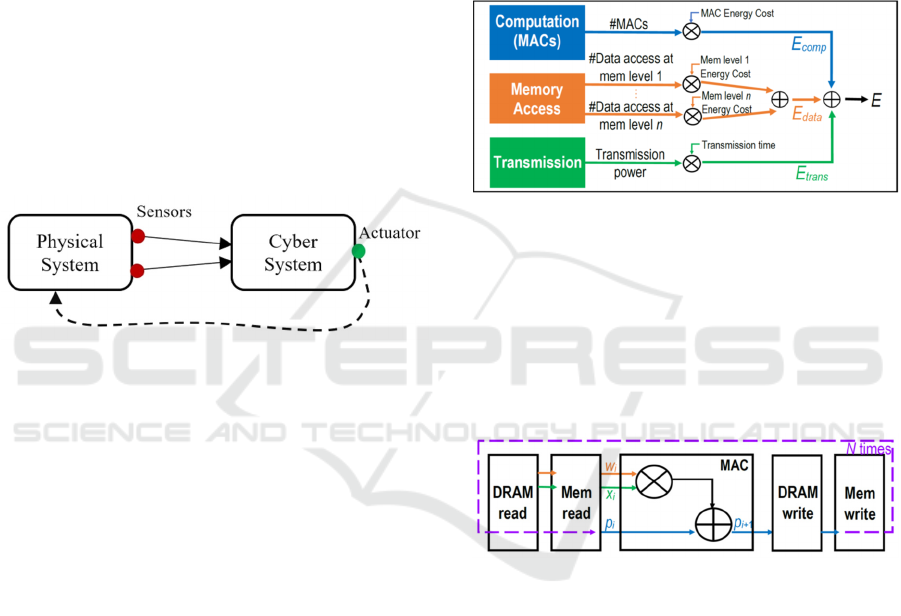
Figure 1 shows a conceptual architecture of CPS,

where cyber and physical systems are tightly

integrated. The physical system sends data to the

cyber system (via sensors). The cyber system takes

sensed data as inputs and computes and produces

output to the physical system (via actuator). The

interactions can be intensive and may be required at

different system granularities, thus CPS needs a tight

component integration for efficiency.

Figure 1: Conceptual architecture of CPS

Physical systems (or components/units) include

human engineered systems (e.g., manufacturing,

building) and natural systems (e.g., solar, climate,

habitat, environments) and Cyber (or Software)

systems (or components/units) include computing

artifacts as well as relevant infrastructures (e.g., data

storage and transmission network). We refer to

sensors and actuators as interface devices and use the

term “computing units” and “cyber/software

components” synonymously.

Although some objects are of physical system

(e.g., sensors, network cables), in estimating energy

consumption of computing units in a CPS, we include

energy consumption consumed by relevant physical

components in computation and data transmission (or

communication). Thus, energy consumption includes

energy consumed by a sensor for sensing and

transmitting the data to a server.

In this section, we describe our approach to

estimating energy consumption of computing units in

CPS. We start with the methodology to estimate

consumption per unit in Section 3.1 then present the

estimation of the system in Section 3.2.

3.1 Unit Energy Estimation

Energy consumption of a computing unit consists of:

(1) energy consumed from computation (E

comp

), (2)

energy consumed from the associated data movement

data

) and (3) energy consumed from transmission to

other units (E

trans

), i.e.,

E = E

comp

+ E

data

trans

(1)

Figure 2 summarizes an overall concept of how to

compute E in (1).

Figure 2: Energy consumption methodology of a computing

unit

Details on the modeling the energy from

computation, data access, and transmission are

presented below in Subsections 3.1.1, 3.1.2, and

3.1.3, respectively.

3.1.1 Computation Energy

Figure 3: A MAC operation

The fundamental element of the computation is a

multiply-and-accumulate (MAC) operation (Yang et

al., 2018). Suppose we want to compute

∑

i=0

Figure 3 depicts a MAC operation, where for each

iteration i, two inputs w

and x

are multiplied and the

result is added to the (accumulated) partial sum p

producing an updated partial sum p

i+1

for the next

iteration (or the accumulated sum of the

multiplication pairs so far). This accounts for one

MAC operation in one iteration. Since the final

summation is a result of n iterations of MACs, we say

it takes n MACs. As a result, computation energy

depends on the number of MACs, giving

comp

= αc

(2)

SMARTGREENS 2022 - 11th International Conference on Smart Cities and Green ICT Systems

where c is the number of MACs and α is hardware

energy cost per one MAC operation.

3.1.2 Data Access Energy

For each computation, data of different types (e.g.,

input and output) need to be stored in the memory. In

particular, as shown in Figure 3, each MAC performs

four data accesses, three reads (i.e., two inputs w

and

and one previous accumulated partial result p

) and

one write (i.e., new partial result p

i+1

). Since energy

spent accessing different levels of memory hierarchy

are significantly different, data movement energy

depends on how data moves in the memory hierarchy

(Yang et al., 2018).

Let M be a memory hierarchy level, V be a set of

data types (e.g., input, output, weight), β

be a

hardware energy cost per data access in the memory

level m, a

v,m

be the number of data accesses for data

of type v accessed at memory level m, and p be a

precision in terms of number of bits for data

representation (e.g., 8, 16). We can estimate the

energy consumption corresponding to data movement

based on the number of data accesses and access

location in the memory as shown below.

data

∑∑

v,m

m=1

v∈V

)

Note that we express β

cache

and β

DRAM

in terms of

energy cost of a MAC operation α, resulting in β

cache

= 6α and β

DRAM

= 200α, used in (Yang et al., 2018).

In this study, without loss of generality, we

consider data moves between two memory levels:

cache (m = 1) and DRAM (m = 2) with a cache hit

rate h. Data are looked up in the cache first. If they

are not found (cache miss), they will be fetched from

DRAM and stored in cache. As a result, we can

simplify data movement energy to be as follows.

data

∑

(β

cache

+ β

RAM

(1-h)a

) p

v∈V

)

As seen in (4), in the best-case scenario (h = 1),

all data are fetched from cache, whereas in the worst

case (h = 0), all data have to be fetched from DRAM

as expected.

3.1.3 Transmission Energy

Transmission energy (E

trans

) of a computing unit can

be calculated from transmission power p scaled by

transmission time t (Mo & Xu, 2020; Z. Yang et al.,

2021). The transmission time can be obtained from

dividing the total number of bits to be transmitted s

by the achievable rate r.

trans

= p

= p (

) (5

)

Depending on communication protocols, the

achievable rate r can be calculated differently. For

example, in Frequency Division Multiple Access

protocol (FDMA) (Z. Yang et al., 2021), r can be

achieved by:

r = b log





)

where b is bandwidth, p is transmission power of the

edge node, h is channel power gain and N

is power

spectral density of the Gaussian noise. Similarly, in

non-orthogonal multiple access (NOMA) protocol

(Mo & Xu, 2020), r can be found by:

r = B log 

∑

i=1

∑

n-1

i=1



)

where B is bandwidth, p is transmission power, h is

channel power gain, n is the number of edge nodes

and 𝜎



is a variance for the additive white Gaussian

noise (AWGN).

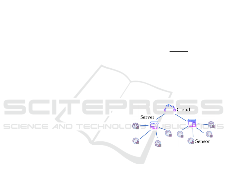
3.2 System Energy Estimation

Figure 4: Sensor-based CPS network

Once we quantify energy for each computing unit as

in Section 3.1, this section combines the energy of all

computing units in a system. Figure 4 shows an

example of a sensor-based distributed system

consisting of two computing units, each is a network

of sensors (or sensing nodes) and distributed server

(or server or edge node). Total energy consumption

of the system can be expressed by

network

ense

erve

(E) (8

)

where N

sense

, N

server

is the number of sensors and

servers, respectively. E

sense

is energy consumed by

each sensing node, which includes consumption

during all sensor operations e.g., sensing, logging and

transmission (Bouguera et al., 2018). Finally, E is

Energy-Aware Deep Learning for Green Cyber-Physical Systems

energy consumed by each server obtained by

modeling approach discussed in the previous section.

4 DEEP LEARNING MODELING

To further explain energy modeling of computing

units in more details (i.e., to show how one can count

the number of MACs and data access in the memory),

we need to work on specific software units. Here we

choose a relatively difficult computing unit of a

popular Deep learning or deep neural network

(DNN). DNN has been widely used in CPS for

various tasks such as control, automation, detection,

and monitoring. This section further describes the

methodology in Section 3.1 to estimate energy of

DNN computation. Specifically, we focus on energy

consumption of computation and data access during

the execution of the trained DNN model on one data

instance. That is, we do not deal with energy usage

for training DNN.

Background of DNN and how to assess the number

of MACs and the number of data access from the

DNN model are described in Subsections 4.1, 4.2, 4.3,

respectively.

4.1 Background on DNN

Artificial neural networks (ANN) are a computational

model consisting of layers of neurons. Each output is

obtained by computing a weighted sum of all inputs,

adding a bias, and (optionally) applying an activation

function as shown in (9). Examples of activation

functions are sigmoid function and Rectified Linear

United (ReLU).

y = f(

∑

+b)

(9)

where y, x

, w

, b and n are the output, inputs, weights,

bias and number of inputs, and f(.) is an activation

function (Sze et al., 2017).

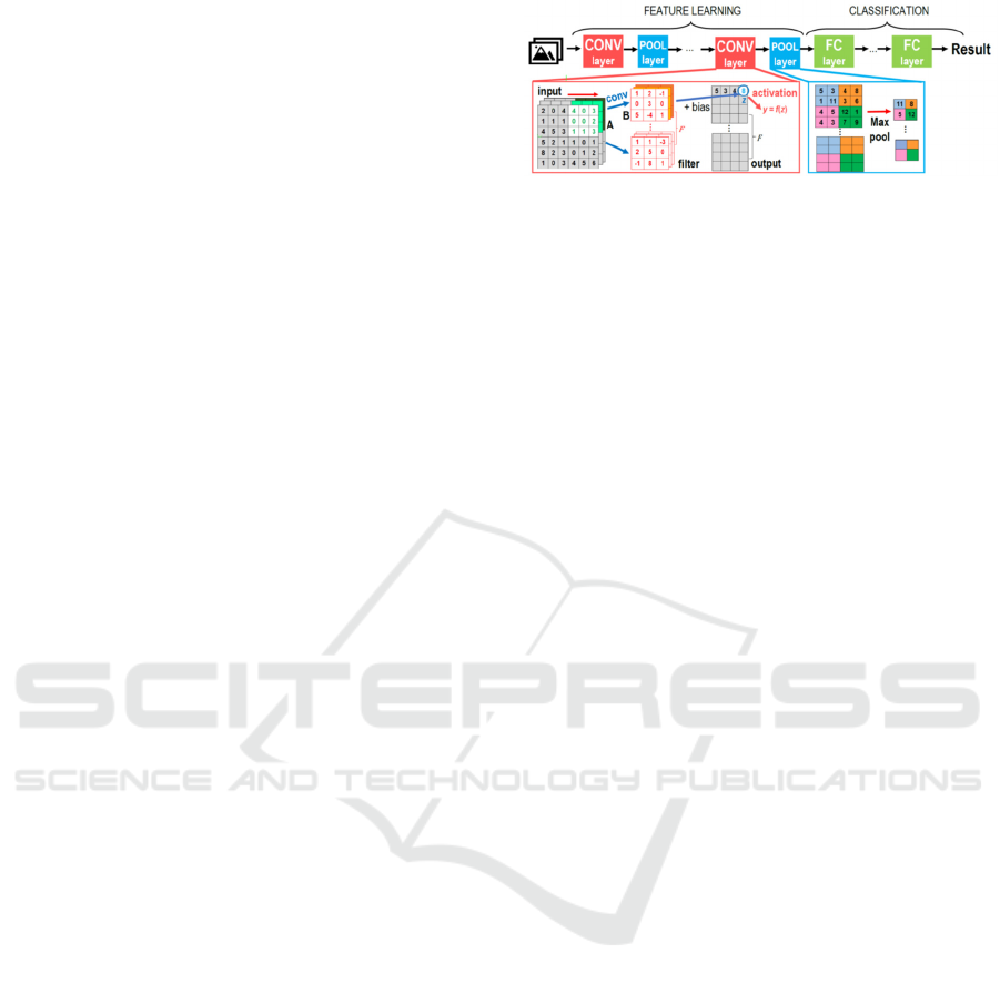
A convolution neural networks (CNN) is a type of

DNN that has been successfully applied to image

analysis and computer vision (e.g., face recognition,

object classification). Figure 5 shows a typical CNN

architecture where multiple convolution (CONV)

layers are used for feature extraction and fully

connected (FC) layers are used for classification.

Since CNN usually deals with images with high

dimensions, pooling (POOL) layers are used to

reduce the dimensionality using pooling operations

(e.g., max, average). As shown in Figure 5, the POOL

layer selects the maximum element of an input region

and reduces dimension of a 4x4 input to a 2x2 output.

Figure 5: A Convolutional Neural Network (CNN)

The CONV layer, a building block of CNN,

consists of high-dimensional convolutions. Equation

(10) defines the computation of each CONV layer.

For each layer, an input (also called input feature

map) is a set of 2-dimensional matrices, each of

which is called a channel. Each channel is convolved

with a distinct filter channel (i.e., 2-dimensional

weights). As seen at the bottom of Figure 5, a

convolution starts with the 2-dim filter slides over a

region of the 2-dim input of the same size, performing

pointwise multiplication and summing the results into

a single value. The convolution results are summed

across all channels (3

dimension of input block).

The bias b can be added to the result, yielding the

single output value z (as shown in (10)).

,m,n

= (

∑∑∑

,c,i,

,c,m+i,n+

) + b

(10

)

where z

s,f,m,n

is the output feature map of layer l, batch

s, channel f and location (m, n), w is the weight of

filter f, channel c and location (i, j), x is the input and

b is bias. The filter repeats this process as it slides

over all the input regions, yielding a filled output

matrix. The process then repeats for all F filters. Each

of the output values (LHS of (10)) then goes through

an activation function and becomes an input to the

next layer (Sze et al., 2017).

Since a DNN model consists of multiple layers of

different types (e.g., convolution, pooling and fully

connected), the total consumption of the DNN is the

summation of computation and data access energy

from all layers. Next, we provide a per-layer

estimation of number of MACs (for computation

energy) and data access (for data access energy)

4.2 Estimation of Number of MACs

Since different type of layers require different

computation, we provide estimation of number of

MACs for each layer as follows.

4.2.1 Fully Connected (FC) Layer

Consider Figure 6 representing a FC layer l of n

neurons, each of which is connected with every

SMARTGREENS 2022 - 11th International Conference on Smart Cities and Green ICT Systems

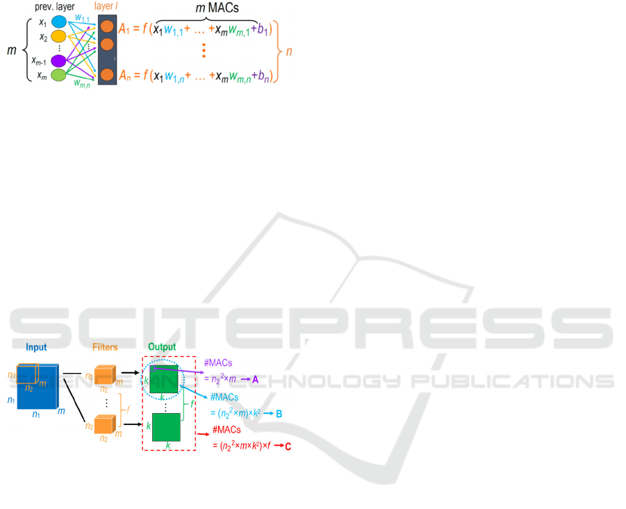
neuron of an FC’s input layer (or previous layer) of m

neurons. (Note that if the FC’s previous layer is a

convolution or pooling layer whose output is

represented in a stack of h 2-dimensional square

planes, say k

k then the input layer of FC has m =

k neurons).

Figure 6: Computation and associated data in FC layer

As shown in Figure 6, for each of n neurons in the

FC layer, we compute m weighted sums (as in f’s

argument) and one activation (by function f). Thus, c,

the total number of MACs in the FC layer is shown

below in (11).

c = mn + c

act

(11)

where c

act

is the number of MACs used in the

activation function which will be determined later.

4.2.2 Convolutional (CONV) Layer

Figure 7: Computation and associated data in CONV layer

The convolution layer aims to extract features by

means of weights in filters. It results in a large number

of computations and corresponding data movements.

An input of n

width and height and m channels is

convoluted with f filters, each of dimension n

x n

m, and results in an output of size k x k x f.

As shown in Figure 7, the convolution process

starts with a pointwise multiplication of a filter and an

input region where the results are summed across all

channels. To obtain this one output value (e.g., the top

leftmost cell of the output), it takes n

m MACs (A in

Figure 7). The convolution process continues for the

rest of the input region, yielding the output of size k

by k yielding the number of MACs (B in Figure 7).

The process then repeats for the rest of the f filters,

ultimately producing f outputs and taking n

MACs, shown as C. Note that the output value can go

through to an activation function which takes another

act

MACs. In other words, to obtain each output

value, it takes n

m and c

act

MACs. The operation

repeats k

f time for all output values giving the total

number of MACs in the CONV layer as:

c = (n

m)(

) + c

(

) (12)

4.2.3 Pooling Layer

The energy consumption of a pooling layer depends

on the type of the pooling operation. We consider the

two popular types: max pooling and average pooling.

In max pooling, the filter slides over input region,

the maximum element in the region is selected as an

output value. Since no MAC operation is used, we

obtain c = 0.

Similar operation is done in average pooling, but

instead of selecting the maximum value of the input

region, the operation averages the values in the

region. Each operation is estimated to use one MAC.

Since the number of pooling operations in a layer is

equal to the size of the output, number of MACs

operation can be expressed as:

c = n

m (13

)

4.2.4 Activation Functions

We estimate computation of different activation

functions in terms of number of MACs to be used in

the earlier layer-wise analysis. We denote c

act

number of MACs required to compute an activation

function.

1. Linear function: f(z) = z requires no MAC giving,

act

= 0.

2. Sigmoid function: σ(z)= 1/(1+e

-z

) takes one MAC

(for a division) with extra computation γ for

exponential function. This gives c

act

= 1 + γ.

3. ReLU function: R(z) = max(0,z). It is a non-linear

function and is widely used in both convolutional

layer and fully connected layer. The computation

does not require MAC, giving c

act

= 0.

4. Softmax function: S(z) = e

∑

i=1

), where m is

a number of classes. The function is typically used

in the output layer for classification. We estimate

the number of MACs to be m+1 (m for product

sum and one for a division) with extra computation

γm (i.e., γ for each of m computations of

exponential function). As a result, we get

act

= 1 + m

+ γm.

Energy-Aware Deep Learning for Green Cyber-Physical Systems

4.3 Estimation of Number of Data Access

Since computation in each type of layers differs,

number of data access also varies. Therefore, we

provide estimation of number of data access for each

layer as follows.

4.3.1 Fully Connected (FC) Layer

For data movement energy in FC layer, we consider

m input neurons, mn weights, n biases and n neurons

in FC layer (or output layer). Let a

be the number of

data accesses for x. As shown in computation of A

’s

in Figure6, each input x

is read n times while each

weight and each bias are each read once. Thus, a total

number of data accesses for input, weight and bias

would be mn, mn, and n, respectively. These results

are shown in (14)-(16). As shown in Figure 6, each

output A

includes read/write accesses of m products,

yielding 2m data accesses. Since there are n output

neurons, a total of number of data accesses for output

would be 2mn as given in (17).

= m(n)

(14)

wei

= m(n)

(15)

bias

= n (16)

out

= n(2m)

(17)

Next section shows how to compute MACs and

data movement energy in CONV layers.

4.3.2 Convolutional (CONV) Layer

Data movement energy in this layer involves input,

filters (i.e., weights), biases and output. As shown in

Figure 7, each input data is accessed at least once for

each filter requiring

m MACs. As the filter slides

over the input, some of the input data are being

accessed again (i.e., being reused). Let t be the

maximum bound of the number of reuses and r

be the

number of data that are reused i times. Thus, for f

filters, number of input data accesses is shown in (18).

Similarly, each weight in the filter and each bias is

accessed once to calculate one output value. To

complete the output for one filter of size k

, as circled

in blue in Figure 7., the weights and bias hence are

accessed k

times. Since there are n

m weights and 1

bias for one filter, with f filters, total number of

weight and bias data access can be expressed in (19)

and (20), respectively. As labeled as A in the Figure

7, each of the output value takes n

m iterations of

MAC. This means the output value is being accessed

2 n

m times accounting for data read and write.

Since there are k

f output values, number of output

data access can be expressed as shown in (21).

= (n

∑

i=2

) · f

(18

)

wei

= n

m f k

(19

)

bias

(20

)

out

= k

f (2n

(21

)

4.3.3 Pooling Layer

Data movement energy for max pooling and average

pooling involves only input and output. The input

data access depends on the size of the filter (i.e.,

pooling size) and stride. Similar to how (18) is

obtained, number of input data access can be

determined by (22). In addition, stride is sometimes

set to be equal to the size of the filter. As a result, the

input region is not overlapped, causing each the input

value to be accessed only once. In this case, the

second term of (23) is zero. In this layer, each output

data is accessed once, which accounts for data write.

= (n

∑

i=2

)

(22

)

out

= n

(23

)

where n

is the width and height of the input, m is

number of channels, n

is the width and height of the

output. Note that, n

is derived from the input, pooling

size k and stride s (i.e., n

= (n

 k/s) + 1).

5 ILLUSTRATIONS

This section illustrates how the model can be applied

in practice to help the design and management of

CPS, particularly in a smart agriculture system.

Section 5.1 describes the system and the unit under

study. Section 5.2 gives experiments and results.

5.1 Smart Agriculture Systems

Smart agriculture systems include smart farming and

smart CPS for controlled environments for precision

agriculture and food security supply (Rajasekaran &

Anandamurugan, 2019). These systems typically

employ sensors to collect data from the field and use

them for various tasks (e.g., crop health monitoring,

and management of soil nutrients, pesticides,

fertilizer, and irrigation) to increase the crop yields.

To sustain such a system, one needs to manage cost

derived from energy consumption from computation

in these units.

SMARTGREENS 2022 - 11th International Conference on Smart Cities and Green ICT Systems

Consider a crop health monitoring subsystem of

the smart agriculture CPS. The subsystem includes a

disease detection unit that deploys a trained DNN

model to analyze plant images sent from neighboring

cameras (sensing nodes) in the field. The server in the

disease detection unit executes the DNN model to

detect if the plant has a disease or to classify the

disease type. It then transmits those images with

corresponding results to the cloud for backup and

further analysis or to be alerted by another unit.

Suppose a farm owner wants to expand the farm to

grow more plants, cover larger area with more sensors

and disease detection computing units. This will lead

to higher energy consumption. The farm owner or the

smart agriculture system engineer needs to manage

energy resource constraint as well as appropriate

structures to maximize the overall net gain to the

farm. Planning for resource management to make

such a smart agriculture system sustainable can be

challenging. In this paper, we limit the scope of our

investigation to energy consumptions of computing

units to identify appropriate scale and structure for a

design of a sustainable future system.

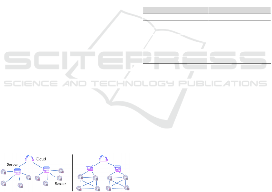
5.2 Experiments and Initial Setup

We consider two CPS network structures: star and

mesh. The left of Figure 8 shows two stars, each of

which has four sensing nodes, where each directly

connects to its assigned distributed server. The right

of Figure 8 shows two meshes, each of which also has

four sensing nodes, all of which are directly

connected to one another. Sensing nodes sense and

transmit their own data but also serve as repeaters that

relay data from other nodes. For examples, sensing

nodes that are not connected to the distributed server

will send their data to their neighbors which will

forward the data to the distributed server. Distributed

servers in both structures connect to the cloud to store

their data.

Figure 8: Star and Mesh Topology.

Since in each star or mesh 80% of nodes are

sensing nodes and 20% of nodes are distributed

server, we use the same ratio between sensing nodes

and distributed servers when we scale total number of

nodes from 100 to 10,000 nodes in our experiments.

Note that each star or mesh maintains 4 sensing nodes

and one distributed server. From this point on, we use

server to mean distributed server, unless it is

specified differently.

For a deep learning model deployed at the server

of each structure, we choose Alexnet (Krizhevsky et

al., 2017), a CNN model to be deployed at the server

due to its popularity and successful use in many smart

agriculture applications (Gikunda & Jouandeau,

2019). Alexnet’s architecture contains 5 convolution

layers with ReLu activation, 3 pooling layers and 3

fully connected layer with Softmax for classification.

In our illustration, data are fetched from cache and

DRAM at 50% cache hit rate. Data precision is 16

bits. The energy consumption is expressed in terms of

the number of MAC operations as it directly

translates to energy usage. We also assume that each

MAC operation consumes about 10 pJ (picojoules).

Table 1: Experimental Setup.

Variable Type/Values

Structure Star, mesh

DL model Alexnet (CNN model)

Data Access Cache (hit rate), DRAM

Communication Protocol FDMA

% No. Servers 20%

% No. Sensors 80%

Bandwidth 500k Hz and 2M Hz

For a communication protocol, we use FDMA

(Frequency Division Multiple Accesses) (Z. Yang et

al., 2021). Bandwidth is set to 500k Hz and 2MHz to

represent low and normal bandwidth scenarios.

Transmission power for each central server is set to

that of a standard laptop at 32 mW while the sensing

node’s is halved (16 mW). Distance between nodes is

set to 100. For sensor energy consumption, the power

and sensing time are 10.5 mW and 25 ms as reported

by (Bouguera et al., 2018). The frequency of the

operation (i.e., the sensing node captures picture and

transmits the data) is set to be every hour. A summary

of experimental setups is shown in Table 1.

Three sets of experiments are performed to help

gain understanding of sources of energy consumption

of the computing units of the smart agriculture

system. The designer of the crop health monitoring

units might ask the following: (1) Does different

structure matter to energy consumption? (2) How

does the number of sensors in each structure effect

energy consumption? (3) Which of the task between

computation or communication consumes more

energy? (4) How much does the bandwidth effect

total energy consumption? Our experiments aim to

answer these questions with respect to scales (i.e.,

number of nodes) of the smart agriculture system.

Energy-Aware Deep Learning for Green Cyber-Physical Systems

6 EXPERIMENTAL RESULTS

The results of the experiments along with some

explanations are discussed in three sections below.

The results should help the farm owner or the smart

agriculture system engineer in designing and

selecting appropriate structures and scale to sustain

energy usage of the new smart disease detection

computing units.

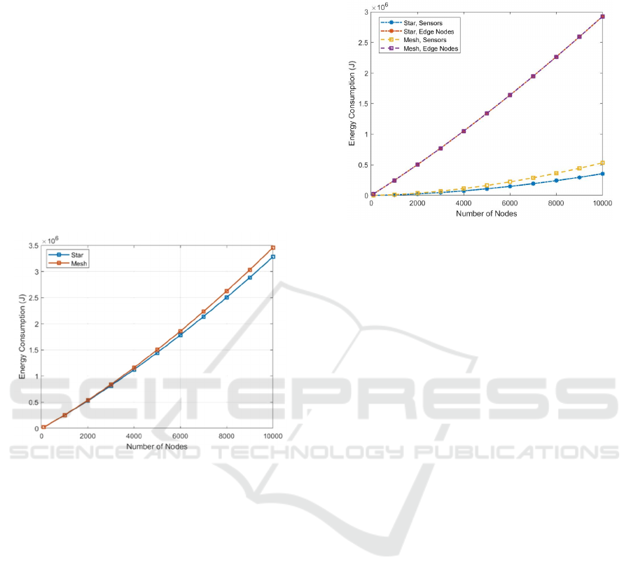
6.1 Effects from Network Structures

We use our analytical energy model to estimate

energy consumptions of two structures: star and mesh

when scaling the number of nodes (i.e., sensors and

distributed servers) up to 10,000 nodes.

Figure 9: Energy consumption of star and mesh networks.

As shown in Figure 9, as we increase number of

nodes, energy consumption linearly increases for both

structures (or topologies) as expected as execution of

each unit requires approximately the same energy

usage in a normal situation (i.e., no transmission

delays). However, the mesh structure consumes

slightly higher energy consumption than the star

structure. This is due to the differences in energy

consumption by data transmissions to be investigated

in more details below.

Figure 10 compares energy consumed by sensing

nodes and (distributed) servers (or edge node) of both

star and mesh structure. In both topologies, shown in

Figure 10, the servers consume significantly higher

energy than the sensors. This is mainly due to high

energy consumption from deep learning execution.

Moreover, as shown in Figure 10, energy

consumption at the servers in both topologies are the

same. This is because the servers in both topologies

perform approximately the same amount of deep

learning computation and transmit the same amount

of data.

Figure 10: Energy consumption of sensors vs. distributed

servers (edge nodes).

On the other hand, Figure 10 shows that the

transmission (or communication) energy at sensing

nodes of the mesh is higher than that of the star. As

the number of nodes increases, the differences in

transmission energy grow. This is because, as

opposed to direct transmission in the star structure,

sensing nodes in the mesh that are not connected to

its designated server require multi-hop transmission.

Since some nodes need to send not only their data but

also data from other nodes, more energy is consumed.

Consequently, the mesh structure has higher

transmission energy and higher total energy

consumption. In our experiments, we consider at most

2-hop data forwarding as depicted in Figure 8. If more

hops are needed to reach the distributed server, even

higher energy consumption is expected.

In general, despite being simple and cheaper in

terms of energy, the star structure has limitation in the

maximum transmission range between the sensing

node and the server. Since sensing node and the

server must be in transmission coverage of one

another, having more sensing nodes may not mean

increased coverage area. Using communication

technology such as LoRa can overcome this issue as

it enables long range transmission with low power

consumption, but it has a low bandwidth. Mesh

topology does not have the same issue as the sensing

nodes can relay data from other nodes and hence can

be anywhere as far as they are connected to another

node. Moreover, it can provide better reliability since

data can be rerouted using different paths in case a

node fails. The smart farming designer has to take

these tradeoffs into consideration along with energy

consumption effects.

SMARTGREENS 2022 - 11th International Conference on Smart Cities and Green ICT Systems

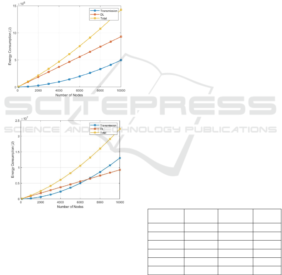
6.2 Effects from Bandwidths

This section explores impact of bandwidth to energy

consumption by computing units. Since the results

between star and mesh networks are similar, we only

show the results from the star network here. We focus

on energy consumption by the distributed servers

rather than sensors since their energy consumption

has much higher contribution to the overall system.

Figure 11 and Figure 12 shows energy consumption

of the distributed server with bandwidth capacity of

2MHz and 500kHz, respectively.

Figure 11: Energy consumption where bandwidth is 2MHz.

Figure 12: Energy consumption where bandwidth is 500kHz.

As shown in Figure 11, with a high bandwidth of

2 MHz, deep learning energy consumption dominates

that of data transmission. Also, total energy

consumption contributed by the DL computation and

data transmission of the distributed server is scalable.

However, this is not the case with a lower bandwidth.

As shown in Figure 12, when there are more than

7,000 nodes, transmission energy starts to dominate

deep learning computation energy. This is because

bandwidth is shared among the nodes. When there are

nodes, higher traffic is expected. This results in

longer transmission time and thus higher energy

consumption. Thus, in the scenario of this experiment

with low bandwidth, the system should not grow

more than 7000 nodes, otherwise, more energy will

be wasted on transmissions instead of actions to gain

productivity (i.e., more images being analyzed). For

the system designer, the ability to estimate energy

consumption per computing units prior to

implementation can give insights on the scale of the

smart farm system to fit the energy budget constraint

or to determine investment on bandwidth capacity.

6.3 Effects from Sensors and Servers Ratios

Results obtained in Section 6.1 indicate that

structures (i.e., mesh, star) of the computing units do

not appear to impact energy consumption that much.

In our previous experiments, the number of sensors in

each structure is set to be four. We want to investigate

further the number of sensors in each structure

impacts energy consumption. This section considers

only the star structure as it is baseline energy

consumption of the two structures.

We consider two sets of sensors, 10 and 100.

Table 2 shows comparison of energy consumption

between having ten and a hundred sensors sending

data to one server. The ratio difference in the last

column represents the ratio of energy consumption in

the 100-sensor case over that in the 10-sensor case.

Thus, it gives a multiplying factor of the former to the

latter. As shown in the first line of Table 1, since the

number of sensors increases 10 times, sensing energy

consumption increases 10 times as expected.

Similarly, at the distributed server, more number of

sensors means more number of images being

processed. Thus, the server has to do 10 times more

image analysis and thus, the energy consumption of

DL execution increases 10 times as it should be.

Table 2: Effect of number of sensors in a star-structured group.

Energy

Consumption

10 sensors +

1 edge node

100 sensors +

1 edge node

Ratio

Difference

Sensing 0.06 0.63 10.00

Sensor Transm. 173.06 2,376.75 13.73

Total at Sensor 173.13 2,377.38 13.73

DL execution 11,624.73 116,247.29 10.00

Edge Transm. 181.67 3,003.42 16.53

Total at Server 11,806.40 119,250.71 10.10

Nevertheless, transmission cost does not

necessarily increase linearly. Transmission energy of

the 100-sensor case is about 13.7 times more than that

Energy-Aware Deep Learning for Green Cyber-Physical Systems

of the 10-sensor case. This is due to higher traffic

which in turns increases the latency and energy.

Similarly, the transmission cost at the server is over

16 times more expensive. Since the server transmits

larger data size than the sensors, this causes heavier

transmission traffic and results in much higher energy

consumption. With the results shown here we make a

conjecture that the number of sensors in each

structure can lead to larger difference of energy

consumption produced by mesh and star topologies.

Overall, our experiments and results aim to show

methodology to help the farm owner or engineer

design a sustainable smart farming system based on

estimated energy consumption of computing units.

7 LIMITATION AND DISCUSSION

This paper focuses on a method for quantifying the

energy consumption of software artifacts in CPS and

illustrates its use for deep learning software. The

evaluation of the resulting models of the deep

learning software are limited to theoretical models.

Proper evaluation of the resulting models requires

further empirical work on real-world systems. This is

beyond the scope of our work in this paper. However,

we show initial findings of our theoretical evaluation

of our resulting models below.

Table 3: Alexnet computation energy.

Method CONV FC Total

Ours 666M 58.6M 724M

Sze et al., 2017 666M 58.6M 724M

T. J. Yang et al., 2018 528M 58.6M 586M

Specifically, we compared energy consumed by

Alexnet and compared with published results in (Sze

et al., 2017) as well as those obtained by an online

analytical tool (T. J. Yang et al., 2018).

In Table 3, assuming that the data movement of the

computation in all the three methods are the same, the

energy consumptions are compared based on the

number of MACs. As shown in Table 3, our results

match those reported by Sze et al. The estimates from

Yang et al., however, are about 21% less than those

of ours and Sze et al.'s. This preliminary result gives

a theoretical comparison of our models with existing

work.

However, to complete the theoretical evaluation,

we need to relax the assumption on data movement.

To fully evaluate our approach, we need to

experiment our method with different software

computation in CPS and obtain energy models to be

compared with actual energy obtained by power

measuring tools in real systems. These are potentials

of our future work.

8 CONCLUSIONS

This paper presents an analytical approach to

quantifying energy consumption of software artifacts

in CPSs. For clarity and due to the increasing use of

deep learning in CPSs, the approach is described

using the deep learning computation process. While

the model is specific to deep learning in distributed

networks, the proposed approach provides a building

block concept that is general in that it can be applied

to any software computation (e.g., other machine

learning or data analysis algorithms) in the CPS other

than deep learning. The paper also illustrates how the

resulting energy model can be applied in practice

including methodology in analyses to help the design

and management of CPS. This contributes to a

fundamental approach towards the development of

green computing CPS, particularly in the aspects of

planning of energy resources.

Future work includes (1) applying the proposed

approach to other real-world CPS software

components, and (2) expanding the energy

consumption modelling to manage CPS resources in

multiple contexts (e.g., economy, energy,

computation, quality of service, environment, and

sustainability).

REFERENCES

Bouguera, T., Diouris, J., Chaillout, J., & Andrieux, G.

(2018). Energy consumption modeling for

communicating sensors using LoRa technology. 2018

IEEE Conference on Antenna Measurements &

Applications (CAMA), 1–4.

Dhaini, M., Jaber, M., Fakhereldine, A., Hamdan, S., &

Haraty, R. A. (2021). Green Computing Approaches-A

Survey. Informatica, 45(1).

Estevez, C., & Wu, J. (2017). Chapter 15 - Green Cyber-

Physical Systems. In H. Song, D. B. Rawat, S. Jeschke,

& C. B. T.-C.-P. S. Brecher (Eds.), Intelligent Data-

Centric Systems (pp. 225–237). Academic Press.

Faviola Rodrigues, C., Riley, G., & Luján, M. (2018).

SyNERGY: An energy measurement and prediction

framework for Convolutional Neural Networks on

Jetson TX1. Proceedings of the International

Conference on Parallel and Distributed Processing

Techniques and Applications (PDPTA), 375–382.

Fu, H., Sharif-Khodaei, Z., & Aliabadi, M. H. F. (2019). An

energy-efficient cyber-physical system for wireless on-

board aircraft structural health monitoring. Mechanical

Systems and Signal Processing, 128, 352–368.

SMARTGREENS 2022 - 11th International Conference on Smart Cities and Green ICT Systems

Gikunda, P. K., & Jouandeau, N. (2019). State-of-the-Art

Convolutional Neural Networks for Smart Farms: A

Review. Advances in Intelligent Systems and

Computing, 997, 763–775.

Haseeb, K., Ud Din, I., Almogren, A., & Islam, N. (2020).

An Energy Efficient and Secure IoT-Based WSN

Framework: An Application to Smart Agriculture.

Sensors, 20(7).

Horcas, J. M., Pinto, M., & Fuentes, L. (2019). Context-

Aware Energy-Efficient Applications for Cyber-

Physical Systems. Ad Hoc Networks, 82, 15–30.

Hossain, M. S., Rahman, M. A., & Muhammad, G. (2020).

Towards energy-aware cloud-oriented cyber-physical

therapy system. Future Generation Computer Systems,

105, 800–813.

Inderwildi, O., Zhang, C., Wang, X., & Kraft, M. (2020).

The impact of intelligent cyber-physical systems on the

decarbonization of energy. Energy \& Environmental

Science, 13(3), 744–771.

Krizhevsky, A., Sutskever, I., & Hinton, G. E. (2017).

ImageNet Classification with Deep Convolutional

Neural Networks. Commun. ACM, 60(6), 84–90.

Li, D., Chen, X., Becchi, M., & Zong, Z. (2016). Evaluating

the Energy Efficiency of Deep Convolutional Neural

Networks on CPUs and GPUs. 2016 IEEE

International Conferences on Big Data and Cloud

Computing (BDCloud), Social Computing and

Networking (SocialCom), Sustainable Computing and

Communications (SustainCom) (BDCloud-SocialCom-

SustainCom), 477–484.

Liang, Y. C., Lu, X., Li, W. D., & Wang, S. (2018). Cyber

Physical System and Big Data enabled energy efficient

machining optimisation. Journal of Cleaner

Production, 187, 46–62.

Mitchell, W., Westberg, S., Reiling, A., Taha, T., Balster,

E., & Hill, K. (2018). Generalized Power Modeling for

Deep Learning. NAECON 2018 - IEEE National

Aerospace and Electronics Conference, 391–394.

Mo, X., & Xu, J. (2020). Energy-Efficient Federated Edge

Learning with Joint Communication and Computation

Design.

Ortiz, J. H., Varela, F. V., & Ahmed, B. T. (2020). Energy

Consumption Model for Green Computing. In Mobile

Computing. IntechOpen.

Rajasekaran, T., & Anandamurugan, S. (2019). Challenges

and Applications of Wireless Sensor Networks in Smart

Farming—A Survey BT - Advances in Big Data and

Cloud Computing (J. D. Peter, A. H. Alavi, & B. Javadi

(eds.); pp. 353–361). Springer Singapore.

Sze, V., Chen, Y. H., Yang, T. J., & Emer, J. S. (2017).

Efficient Processing of Deep Neural Networks: A

Tutorial and Survey. Proceedings of the IEEE, 105(12),

2295–2329.

Yang, T. J., Chen, Y. H., Emer, J., & Sze, V. (2018). A

method to estimate the energy consumption of deep

neural networks. Conference Record of 51st Asilomar

Conference on Signals, Systems and Computers,

ACSSC 2017, 2017-Octob, 1916–1920.

Yang, Z., Chen, M., Saad, W., Hong, C. S., & Shikh-

Bahaei, M. (2021). Energy Efficient Federated

Learning over Wireless Communication Networks.

IEEE Transactions on Wireless Communications,

20(3), 1935–1949.

Yu, B., Zhou, J., & Hu, S. (2020). Cyber-physical systems:

An overview. Big Data Analytics for Cyber-Physical

Systems, 1–11.

Zeng, D., Gu, L., & Yao, H. (2020). Towards energy

efficient service composition in green energy powered

Cyber–Physical Fog Systems. Future Generation

Computer Systems, 105, 757–765.

Zhu, S., Ota, K., & Dong, M. (2021). Green AI for IIoT:

Energy Efficient Intelligent Edge Computing for

Industrial Internet of Things. IEEE Transactions on

Green Communications and Networking, 1.

Energy-Aware Deep Learning for Green Cyber-Physical Systems