Demand-responsive Scheduling in Railway Transportation

Christoph Gr

une

1 a

and Stephan Zieger

2 b

Department of Computer Science, RWTH Aachen University, Aachen, Germany

Institute of Transport Science, RWTH Aachen University, Aachen, Germany

Keywords:

Integer Programming, Railway Scheduling, Demand-responsive Transport, Rural Railway Networks, Dial-a-

Ride, Timetabling.

Abstract:

Rural rail transportation can contribute signiﬁcantly to achieving climate goals and encountering mobility

challenges, especially by reactivating currently disused railway lines. Rural areas are mainly characterised

by their dispersed demands. Thus, small highly automated rail vehicles could be operated on-demand and

thus service-oriented. The operation of those networks is complex and the economic efﬁciency must be corre-

spondingly high. Therefore, optimised resource planning is necessary. The paper focuses on the planning of

a-priori known transport requests.

The paper presents a formulation for the underlying Integer Programming mathematical model that optimises

travel times and number of vehicles used under consideration of railway speciﬁc constraints such as headway

times and deadlock prevention. The modelling goes beyond existing Dial-a-Ride approaches and adds the nec-

essary routing constraints for rail systems as well as energy management constraints for potential refuelling or

recharging.

The potential for application of the approach is evaluated in a computational study. A validation scenario

shows in an exemplary manner on the one hand how the constraints affect routing on a single track railway

line and on the other hand how solving the model with a black-box solver such as Gurobi is handled for this

scenario. On a real-world railway line, it can be shown that the Integer Programming solver is able to induce

meaningful results for limited input sizes. Further potential improvements are discussed as well.

1 INTRODUCTION

The Commission of the European Union (European

Commission, 2020) identiﬁed several mega trends

that will inﬂuence general life in the coming decades.

These include challenges such as climate change, ur-

banisation, the ageing population as well as transport

and behavioural changes. In order to mitigate or even

avoid the consequences, the strengthening of the rail-

way system is an essential factor. Especially in rural

areas, transport services are often poor, non-existent

or discontinued. As demand in rural areas is usually

much lower and more dispersed, smaller automated

rail vehicles are a viable option such as the ANT sys-

tem proposed by Siemens (Schlaht et al., 2018) or

the Aachen Rail Shuttle (Schindler and von Stillfried,

2020).

These small automated trains can operate on a

demand-responsive basis, thereby improving both ac-

https://orcid.org/0000-0002-7789-8870

https://orcid.org/0000-0003-4936-0018

cessibility and availability of public transport. In this

paper, technical and legal challenges are assumed to

be solved and the focus is on operational questions.

The emphasis here is on the scheduling, routing and

energy management of the vehicles. In contrast to

road transport, rail transport has some other types of

constraints. The degrees of freedom in rail transport

are often lower, but the dependencies are signiﬁcantly

higher.

1.1 Our Contribution

Our main contribution is the integrated modelling

of scheduling, routing and energy management con-

straints in the railway setting. This integration of the

various constraints goes beyond existing approaches

which are often solved as stages, as discussed in the

Problem Statement. Especially the routing is much

more relevant and complicated in the railway setting

as several constraints such as headway times or dead-

lock prevention are rather speciﬁc and much more rel-

Grüne, C. and Zieger, S.

Demand-responsive Scheduling in Railway Transportation.

DOI: 10.5220/0011018700003191

In Proceedings of the 8th International Conference on Vehicle Technology and Intelligent Transport Systems (VEHITS 2022), pages 239-248

ISBN: 978-989-758-573-9; ISSN: 2184-495X

239

evant.

We develop a model to tackle the overall problem.

With this modelling, effects of infrastructure expan-

sion or the size of the vehicle ﬂeet can be quanti-

ﬁed by using the modelling as a black box. Thus,

different infrastructure variants in combination with

the optimal scheduling solution can be used as a deci-

sion support tool for the implementation of a demand-

responsive railway system.

In the main model, the number of vehicles and re-

quests are ﬁxed and all requests must be served. Fur-

ther objective variants enable for example maximising

the number of passengers served with the available re-

sources. This is relevant when the number of vehicles

is ﬁxed and often there are a few requests which have

extraordinary costs for fulﬁlling. Another variation

of the objective function is minimising the number of

used vehicles while still fulﬁlling all requests. Here,

the service quality is of importance, but the reduction

of costs for the acquisition of the vehicles is the main

objective.

1.2 Related Work

The Dial-a-Ride Problem (DARP) has a long stand-

ing history (Stein, 1978). It is a special routing and

scheduling problem in which the users specify re-

quests for their pick-up and drop-off at their origin

and destination, respectively. The objective is usually

to compute a schedule fulﬁlling several constraints

and maximising the number of transported persons

while minimising the costs doing so. Cordeau and La-

porte (Cordeau and Laporte, 2003; Cordeau and La-

porte, 2007) as well as Ho et al. (Ho et al., 2018)

provide an excellent overview on model variants and

solution techniques.

In contrast to the also well-studied Periodic Event

Scheduling Problem (Seraﬁni and Ukovich, 1989;

Liebchen and M

ohring, 2007) which has many ap-

plications in railway scheduling the DARP is char-

acterised by its irregular requests and corresponding

scheduling. The DARP has been studied mainly for

rubber-tyred systems. Railway systems offer less de-

grees of freedom in terms of moving directions for

example compared to cars. However, the degree of

interdependence is much stronger, e.g. on single track

lines (Szpigel, 1973; Landex, 2009). Several schedul-

ing approaches by means of Integer Programming ex-

ist for the railway scheduling problem (Castillo et al.,

2009; Castillo et al., 2011; Caimi et al., 2017), but

their scope is often limited and concern the construc-

tion of schedules on main lines or improve dispatch-

ing decisions (Weik et al., 2018; Li et al., 2013).

Cats and Haverkamp (Cats and Haverkamp, 2018a;

Cats and Haverkamp, 2018b) assume an automated

demand-repsonsive rail service on main lines and de-

termine the optimal line and station capacity for such

a system. To the best of the authors knowledge this is

the only related work in this setting.

1.3 Outline

The paper’s structure is as follows. In the Prelimi-

naries, the graph representation of the railway infras-

tructure is presented. Following, the problem is stated

informally. In Sec. 3, the main part of the paper, the

model is proposed by means of Integer Programming

and different variants are discussed. Subsequently, a

computational study (Sec. 4) is performed in which

ﬁrst a validation scenario is investigated and after-

wards a real railway line are subject to the study. Fi-

nally in Sec. 5, the paper is summarised and an out-

look on further open work is discussed.

2 PRELIMINARIES

In the beginning, the abstraction from real-world rail-

way infrastructure to a graph is described. The ab-

straction is necessary to use models which will then

be able to provide decision support for real-world in-

stances. In the end of the section the problem is stated

informally.

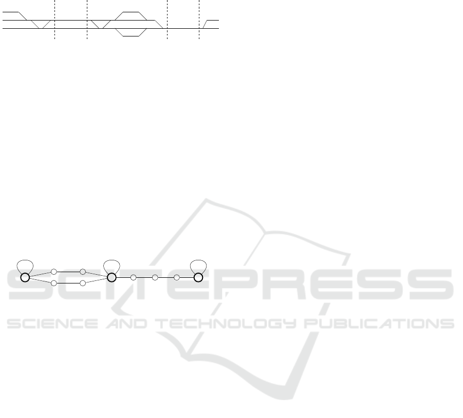
2.1 Railway Network Modelling

The railway network consists of several components

and can basically be divided into the line section and

stations as denoted in Fig. 1. The stations are char-

acterised by their capacity for dwelling and the possi-

bility of boarding and alighting passengers. The line,

in turn, is located between two stations and is usu-

ally single or double track. Speciﬁcally, in rural ar-

eas, the lines are often single track. Depending on

the underlying protection system, the lines are often

divided into blocks based on the placement of sig-

nals. This segmentation is therefore often modelled

as several sections of the line. Due to the compar-

atively high number of individual train movements,

which strongly stress the capacity, and the technical

possibilities with the use of automated vehicles, a re-

duction of the block sizes is to be aimed for. In this

way, headway times of trains are kept as short as pos-

sible and the capacity is used in the best possible way.

In fact, the use of automated and connected vehicles

likely results in minimum headway times in the realm

of the relative braking distance, i.e. just a few seconds

VEHITS 2022 - 8th International Conference on Vehicle Technology and Intelligent Transport Systems

240

for homogeneous vehicles, and is assumed in the fol-

lowing.

Station

Line

Station

Line

Station

Figure 1: Rail infrastructure with three Stations and a

double-track line as well as a single track line between

those.

The abstraction of the infrastructure is performed

by the introduction of a graph G = (V, E). In Fig. 2 the

exemplary transformation for the infrastructure from

Fig. 1 is depicted. In this graph, the set of vertices

V represents the beginning/end of a block section and

especially the station entrance/exit, i.e. switch areas.

The edge set E models the block sections and station

tracks. Generally the edge set is undirected, but if the

direction of movement is relevant, e.g. due to signals

on a double track section, the undirected edges can be

turned into directed arcs. In case the distance between

two stations is longer than one time step, the edge can

be subdivided into a path of appropriate length.

1 1 1 1

4 2

Figure 2: Example mesoscopic infrastructure abstraction by

means of a graph with appropriate edge capacities.

The model is focused on the usage of the edges

and therefore they contain several properties. First

of all, they have a capacity, which is usually one be-

cause, for safety reasons, only one train is allowed to

be within one section at any given time. We abstract

the trains’ pre- and post-occupation of sections as they

are likely to traverse the network as ”moving block”.

In stations, the edge capacity determines the number

of vehicles the station can withhold and can alterna-

tively be modelled as multigraph if all edges should

have capacity equal to one. Additionally, edges in-

clude the information about the travel time on those.

These have to be integer and longer sections are usu-

ally split up such that each edge needs one time step

to be traversed.

2.2 Problem Statement

Usually, the transport planning problem consists of

a series of hard tasks which are often executed one

after each other. These are demand estimation,

line planning, scheduling, platform and track assign-

ment, rolling stock planning, crew scheduling as well

as shunting and maintenance planning (Goossens,

2004). In the case of highly automated unmanned ve-

hicles, the problem reduces to the scheduling, plat-

form and track assignment as well as rolling stock

assignment aspects. In fact, the routing of trains of

capacity greater than one, which is a sub-problem of

this problem, is already NP-hard (Guan, 1998). Thus,

this problem is expected not to be solvable efﬁciently.

The task is to ﬁnd a feasible schedule transport-

ing the passengers directly from origin to destination

while fulﬁlling all routing and energy management

constraints, if possible. The resulting schedule should

minimise the costs, i.e. the number of train move-

ments. Other possible objectives are discussed in

Sec. 3.2. The passengers specify their origin and des-

tination along with some time window each. When

the passengers board or alight, the trains will need to

be assigned some dwell time to give sufﬁcient time

for doing so. The vehicles operated on the network

are constrained by their capacity, i.e. the number

of passengers which can be transported at the same

time, and the energy capacity. Often, rural railway

lines are not electriﬁed and thence the vehicles have

to recharge or refuel after some time.

The railway system is characterised by strong in-

terdependencies. One prime example is the minimum

headway time, i.e. the least amount of time which has

to pass between two successive (or opposing) trains

such that the second train can move unhindered from

the ﬁrst train. The trains therefore need to have sufﬁ-

cient spacing between each other.

3 MIXED INTEGER

PROGRAMMING

FORMULATION

In the following, the problem is to be modelled by

means of an Integer Programming formulation. In

the ﬁrst part, an overview on the notation is given.

Then, the model is presented and the constraints are

explained. Finally, necessary modiﬁcations for differ-

ent objective variants are discussed.

3.1 Model

The relevant notation of the model is summarised in

Tab. 1. The table contains the description of the graph,

sets, parameters and variables.

Illustrating the use of the tracker variables for the

passengers and vehicles, Fig. 3 depicts the states for

passenger p assigned to train r. It can be seen that

each passenger is always in a clearly deﬁned and dis-

Demand-responsive Scheduling in Railway Transportation

241

Table 1: Relevant notation for the model.

G Underlying graph

V (G) Vertex set of graph G

H(G) ⊆ V (G) Station vertex set

D ∈ H(G) Depot vertex

E(G) Edge set of graph G

(G) ⊆ E(G) Station edge (platform) set

∈ E(G) Depot edge

Vehicle Capacity of edge e ∈ E(G)

R Set of all vehicles

P Set of all passengers

T Time horizon

T Set of all timestamps of the discretised interval [0, T ]

s(p) Start station vertex of passenger p ∈ P

(p) Start station edge of passenger p ∈ P

d(p) Destination station vertex of passenger p ∈ P

(p) Destination station edge of passenger p ∈ P

(p) Start time window for passenger p ∈ P

(p) Destination time window for passenger p ∈ P

w Dwell time at stations

L(p) Distance from s(p) to d(p) for p ∈ P

ε Percentage distance extension

c(r) Passenger capacity of vehicle r ∈ R

E(r) Charging speed of vehicle r ∈ R

(r) Energy storage capacity of vehicle r ∈ R

, y

, hd

, ad

Auxiliary variables {0,1}

·,·

, W Big-M-parameters

r,e

Is vehicle r ∈ R using edge e ∈ E(G) at time t ∈

T ? {0,1}

r, p

Is person p ∈ P in vehicle r ∈ R at time t ∈

T ? {0,1}

h, p

Is person p ∈ P at station h ∈ {s(p), d(p)} ⊆ H(G) at time t ∈

T ? {0,1}

r,h, p

Does vehicle r ∈ R dwell for passenger p ∈ P

at stations h ∈ {s(p), d(p)} ⊆ H(G) at time t ∈

T ?

{0,1}

Does vehicle r ∈ R refuel/recharge at time t ∈

T ? {0,1}

r, p

Does vehicle r ∈ R transport passenger p ∈ P? {0,1}

tinct state. In the beginning, they wait for the train,

then they board the train at their origin, travel to their

destination and alight there and, ﬁnally, their request

is completed.

s(p), p

r,s(p), p

r,p

r,d(p), p

d( p), p

p waits for r

p enters r

p travels in r

p disembarks from r

p has arrived

Figure 3: The plot of the 5 tracker variables a

s(p), p

, h

r,s(p), p

r, p

, h

r,d(p), p

, a

d(p), p

Following, the objective and constraints are pre-

sented and explained below.

min

∑

r∈R

∑

e∈E\H

∑

t∈

r,e

(1)

The objective in Eq. (1) minimises the number of used

edges which are not station edges, i.e. travelled dis-

tance of all vehicles is minimised. In consequence,

the vehicles only move if absolutely necessary and

the objective can be understood as the minimisation

of operation costs for the operator given the set of ve-

hicles.

∑

e∈E

r,e

= 1 ∀r ∈ R, t ∈

T (2)

∑

∈N

[e]

t−1

r,e

≥ x

r,e

∀r ∈ R, e ∈ E, t ∈

T \ {0} (3)

Eq. (2) ensures that each of the vehicles is located on

exactly one edge for each time step. Together with

Eq. (3), the vehicles then can only move to adjacent

edges and a ﬂow conservation in the time-expanded

VEHITS 2022 - 8th International Conference on Vehicle Technology and Intelligent Transport Systems

242

graph is enforced. The neighbourhood N

[e] is closed

as vehicles have to be able to wait or dwell, e.g. in

front of switches or in stations while waiting for the

next passenger request.

∑

r∈R

r, p

= 1 ∀ p ∈ P (4)

r,s(p), p

≤ v

r, p

∀r ∈ R, p ∈ P, t ∈

T (5)

r, p

≤ v

r, p

∀r ∈ R, p ∈ P, t ∈

T (6)

r,d(p), p

≤ v

r, p

∀r ∈ R, p ∈ P, t ∈

T (7)

Eq. (4) assigns each passenger to a vehicle such that

all passenger requests have to be served. The follow-

ing three equations (5)-(7) ensure that the tracker vari-

ables h

r,s(p), p

, y

r, p

and h

r,d(p), p

for each passenger and

vehicle pair can only be activated if the passenger is

assigned to the vehicle.

∑

p∈P

r, p

≤ c(r) ∀r ∈ R, t ∈

T (8)

∑

r∈R

r,e

≤ c

∀e ∈ E, t ∈

T (9)

The next two equations are concerning capacities.

Eq. (8) enforces the vehicle’s capacity c(r) not to be

exceeded, i.e. at most c(r) passengers are able to

travel in one vehicle at the same time. The second

part limits the line capacity depending on the avail-

able infrastructure. In the same time step, only one

vehicle is allowed at each line section and therefore

is usually set to one for the open line. This con-

straint ensures a safety distance between two succes-

sive trains which is known as the minimum headway

distance. On a single track line the constraint further-

more prevents deadlocks, i.e. two trains facing each

other without the chance of evasion. In stations, c

denotes the number of vehicles a station can contain

at each step in time.

∑

t∈W

(p)

r,s(p), p

≥ 1 ∀ p ∈ P (10)

∑

t∈W

(p)

r,d(p), p

≥ 1 ∀ p ∈ P (11)

Eqs. (10) and (11) allow the speciﬁcation of time win-

dows for boarding and alighting for each passenger.

With these equations it is possible to map the passen-

gers (dis-)satisfaction with waiting times.

∑

t∈

r, p

≤ (1 + ε)L

∀r ∈ R, p ∈ P (12)

Besides the waiting times, users expect not to take ex-

tended detours between their starting point location

and destination. Eq. (12) allows to deﬁne an accepted

detour factor ε extending the length of the shortest

path L(p).

(r) +

∑

∈[0,t]

(

E(r) f

−

∑

e∈E\E

r,e

) ≤ c

(r)

∀r ∈ R, t ∈

T (13)

(r) +

∑

∈[0,t]

(

E(r) f

−

∑

e∈E\E

r,e

) ≥ 0

∀r ∈ R, t ∈

T (14)

≤ x

r,D

∀r ∈ R, t ∈

T (15)

The Eqs. (13)-(15) are concerned with the charging

process. Each vehicle starts with a full charge c

(r).

Subsequently, exactly

E(r) units of energy can be re-

generated in each charging step ( f ). For simpliﬁ-

cation, only the movement costs one unit of energy.

Eq. (13) ensures that charging does not exceed the en-

ergy capacity c

(r) of a vehicle. At the same time,

Eq. (13) ensures that there is always enough energy.

The last constraint guarantees that the vehicle is at the

depot when it is charging.

s(p), p

= 1 ∀ p ∈ P (16)

s(p), p

= 0 ∀ p ∈ P (17)

r, p

= 0 ∀r ∈ R, p ∈ P (18)

r, p

= 0 ∀r ∈ R, p ∈ P (19)

d(p), p

= 0 ∀ p ∈ P (20)

d(p), p

= 1 ∀ p ∈ P (21)

Eqs. (16)-(21) set the variables which have to be ﬁxed

in the beginning or end. In the beginning (Eqs. (16)-

(17)), the passengers are deﬁnitely waiting at their

starting point location s(p) and will not be waiting

there at the end of the time horizon. Each passenger

p can only be transported in a vehicle r after waiting

at the starting point location s(p) and before reaching

their destination d(p). Therefore, the y-variable is set

to 0 in the beginning and end of the time horizon in

Eqs. (18) and (19). Finally, the passengers are never

located at their destination d(p) at the beginning of

the time horizon, but are deﬁnitely there at the end.

∑

r∈R

∑

t∈

r,s(p), p

≥ 1 ∀ p ∈ P (22)

∑

r∈R

∑

t∈

r, p

≥ 1 ∀ p ∈ P (23)

∑

r∈R

∑

t∈

r,d(p), p

≥ 1 ∀ p ∈ P (24)

Each passenger has to be transported. To ensure that

all necessary variables are at least enabled once dur-

ing the time horizon, Eqs. (22)-(24) enforce setting

each to one for at least one time step. The a-variables

already fulﬁl this demand as per the previous set of

equations.

Demand-responsive Scheduling in Railway Transportation

243

s(p), p

∑

r∈R

r,s(p), p

+ y

r, p

+ h

r,d(p), p

) + a

d(p), p

= 1

∀ p ∈ P, t ∈

T (25)

r,s

(p), p

≥ h

r,s(p), p

∀r ∈ R, p ∈ P, t ∈

T (26)

r,d

(p), p

≥ h

r,d(p), p

∀r ∈ R, p ∈ P, t ∈

T (27)

r, p

≤ 1 − a

t−w

s(p), p

∀r ∈ R, p ∈ P, t ∈

T , t ≥ w (28)

t−w

r, p

≤ 1 − a

t−w

d(p), p

∀r ∈ R, p ∈ P, t ∈

T , t ≥ w (29)

Every passenger has to be in one of the states (wait-

ing at the station before boarding, boarding, driving,

alighting, service ﬁnished) during the time horizon.

Therefore, Eq. (25) enforces one of the corresponding

variables always to be set to one. Eqs. (26)-(27) con-

nect the waiting state of the passenger for boarding

and alighting with the position of the allocated vehi-

cle. This implies the vehicle to move to the boarding

edge, travel with the passenger and stop at the alight-

ing edge as well. The passengers are allowed some

time w for boarding and alighting and Eqs. (28)-(29)

take these constraints into account.

t−1

≤ hs

(30)

∑

r∈R

r,s(p), p

6= 1 + M

(31)

= 1 + M

(1 − h

) (32)

6= 1 + M

(33)

s(p), p

= 0 + M

(1 − h

) (34)

t−1

≤ y

(35)

∑

r∈R

r, p

6= 1 + M

(36)

= 1 + M

(1 − y

) (37)

6= 1 + M

(38)

∀ p ∈ P, t ∈

T \ {0}

r,s(p), p

= 0 + M

(1 − y

) (39)

∀r ∈ R, p ∈ P, t ∈

T \ {0}

t−1

≤ hd

(40)

∑

r∈R

r,d(p), p

6= 1 + M

(41)

= 1 + M

(1 − hd

) (42)

6= 1 + M

(43)

∀ p ∈ P, t ∈

T \ {0}

r, p

= 0 + M

(1 − hd

) (44)

∀r ∈ R, p ∈ P, t ∈

T \ {0}

t−1

≤ ad

(45)

∑

r∈R

d(p), p

6= 1 + M

(46)

= 1 + M

(1 − ad

) (47)

6= 1 + M

(48)

∀ p ∈ P, t ∈

T \ {0}

r,d(p), p

= 0 + M

(1 − ad

) (49)

∀r ∈ R, p ∈ P, t ∈

T \ {0}

Eqs. (30)-(49) introduce many auxiliary variables.

Each 5-tuple of constraints follows the same pat-

tern. The general idea is to ensure that the pas-

sengers are handled in the correct order of variables

s(p), p

, h

r,s(p), p

, y

r, p

, h

r,d(p), p

, a

d(p), p

). In some cases,

e.g. with very loose time windows, the chronological

order of the service is not imposed directly. There-

fore, these additional constraints need to be incorpo-

rated. For the sake of the argument, the general pro-

cedure for each block of constraints is discussed by

means of the ﬁrst set as all of those work the exact

same way. The blocks are written in non-standard

form on purpose for better readability. All transfor-

mation steps are done according to Bisschop (Biss-

chop, 2006, Chap. 7).

First, an auxiliary variable hs

is introduced which

ensures that once the corresponding tracker variable

r,s(p), p

became active the auxiliary variable is always

set to one. The following two constraints state that

if the corresponding tracker variable h

r,s(p), p

is set to

one (A) then the auxiliary variable hs

is set to one as

well (B). From this moment on, hs

will be set to one

even if h

r,s(p), p

is already set to zero again.

Let ¬A and ¬B denote the negation of A and B as

usual. Then the statement ”if A then B” is equivalent

to the logical expression ”(A and ¬B) is false”. The

negation ”¬ (¬A and B)” is then true. This in turn is

equivalent to state ”(¬A or B) is true” which is repre-

sented by Eqs. (31) and (32) using the Big-M-method.

The ﬁnal two equations in this block work the exact

same way and state that if the auxiliary variable hs

is set to to one the previous tracker variable a

s(p), p

cannot be one anymore and will not be so, too. This

ensures that exactly one tracker variable is set to one

for each passenger for each time step.

VEHITS 2022 - 8th International Conference on Vehicle Technology and Intelligent Transport Systems

244

3.2 Variants

The problem as is can be used in different variants

covering different objectives. These also have strong

implications on economic factors and passenger satis-

faction. In the model presented above, all passengers

have to be served and all vehicles could potentially be

used, even if unnecessary, as only the number of used

edges outside the station is relevant and penalised in

the objective function.

First, it might not be possible to serve all request

with the available amount of vehicles. Then, the

model would just return that there exists no feasible

solution. Another approach is to maximise the num-

ber of serviced passengers while still minimising the

costs for doing so. This goal can be achieved by alter-

ing the objective function (Eq. (1)) to

min−W (

∑

r∈R

∑

p∈P

r, p

)

∑

r∈R

∑

e∈E\H

∑

t∈

r,e

. (50)

Some large enough value W ensures that the ﬁrst part

of the sum is always relevant and thus the number of

passengers is indeed maximised.

Second, from an economical point of view it

makes sense to minimise the number of vehicles in

usage. Therefore, one possibility is specifying for

example the number of vehicles equal to the num-

ber of passengers and then ﬁnd out how many vehi-

cles are necessary at all. Therefore, another variable

∈ {0, 1} is introduced indicating if a vehicle is used.

The objective (Eq. (1)) changes to

minW

∑

r∈R

∑

r∈R

∑

e∈E\H

∑

t∈

r,e

(51)

and the following constraint is necessary

∑

p∈P

r, p

|P|

≤ v

∀r ∈ R. (52)

For each vehicle r ∈ R, the number of passengers

r, p

) that have used it is counted and the sum is then

divided by |P|. Since v

is an integer, the variable is

always set to 1 if and only if the vehicle is used and,

by the objective function, to 0 otherwise.

4 COMPUTATIONAL STUDY

In this section, at ﬁrst two scenarios for testing the

implementation of the model are described. One of

them is a pure validation scenario presenting the con-

ﬂict management on single track sections. Next, the

framework of the implementation is presented. Fi-

nally, some results are discussed for the two scenarios

which will be the bridge to the conclusion of the pa-

per.

4.1 Scenario Description

In order to evaluate the solving procedure on the

mathematical programming formulation two different

railway networks are used.

The ﬁrst instance is a simple artiﬁcial infrastruc-

ture of two stations with a short single track line in be-

tween. This infrastructure is used to perform parame-

ter tests and to validate the correctness of the mathe-

matical programming formulation, especially with re-

gard to conﬂict detection and avoidance. In Fig. 4 the

route map can be found. The numbers correspond to

the mileage of the stations.

(0.0) Station 1

(2.0) Station 2

Figure 4: Route map of the validation instance.

Additionally, the solution procedure is tested

against a real-world infrastructure as an illustra-

tive example. The former railway line Solingen–

Wuppertal-Vohwinkel connected the towns Solingen

and Wuppertal, both in North Rhine-Westphalia, Ger-

many. Most of the line is disused, partly even disman-

tled. The 22 km long railway line is mostly single-

track and has 10 stations. Fig. 5 presents a the route

map for this railway line.

(0.0) Solingen Hbf

(4.9) Weyersberg

(5.6) Solingen (Weyersberg)

(6.0) Solingen Gr

unewald

(6.2) Solingen S

(6.8) Solingen Mitte

(8.5) Solingen Nord

(10.1) Solingen-Wald

(15.4) Solingen-Gr

afrath

(22.0) Wuppertal-Vohwinkel

Figure 5: Route map of the railway line Solingen—

Wuppertal-Vohwinkel.

4.2 Framework

The model is the integral part within the procedure

which is implemented in Matlab 2019b (MATLAB,

2020) as a frame. There, the infrastructure and re-

quest generation is performed. The model itself

is written according to the speciﬁcations of ZIMPL

(Koch, 2005) which is then also used to transform

the text model into a machine readable model ﬁle.

Demand-responsive Scheduling in Railway Transportation

245

Then, Gurobi (Gurobi Optimization, 2020) is used

as a solver and the output is evaluated and visu-

alised within Matlab again. The computations are

performed on a machine with an i5-6500@3.2GHz (4

Cores) with 16 GB RAM.

4.3 Results

In the ﬁrst part, some results are presented for the val-

idation scenario and then for the real-world example.

c = 1 c = 1

c = 3 c = 3

(a) Graph representation for the validation

infrastructure.

1 2

Stations

Time

Train 1

Train 2

Train 3

(b) One optimal schedule for the validation

scenario.

0 200 400 600 800

Time [s]

100

Gap [%]

T = 30

T = 20

T = 15

T = 10

windows.

Figure 6: Results for the validation scenario.

The abstraction of the route map can be seen in

Fig. 6a. Assuming that the vehicles travel at an aver-

age speed of about 60 km/h, this results in a distance

of about 1 km per minute. The minute measure also

seems to be a good time length for the time steps in

the following cases. In general, there is a trade-off be-

tween the accuracy of the modelling and the efﬁcient

computability of the solution.

The graph consists of the two stations with self

loops (platforms) and an intermediate node that acts

as a separator for subsequent train runs. To illustrate,

3 passengers are to travel from one station to the other,

respectively, each vehicle can only transport 1 person

and the time window is set to 10 minutes and starts at

time step 0. In Fig. 6b an optimal solution is plotted as

a time-distance diagram. Due to the limited time win-

dow, the requests have to be bundled and processed

directionally one after the other. This allows the trains

to follow each other in the same direction with one

time unit between them. If the trains were to run al-

ternately, two time units would be blocked for each

train.

In Fig. 6c the gaps between the found solution and

the proven lower bound are presented over a maxi-

mum computing time of 15 minutes for the same sce-

nario, but with an increasing time window. It can

be observed that just by increasing the time window

slightly, an optimal solution is found within seconds,

but this cannot be effectively proven by the solver us-

ing the lower bound. Due to the high number of sym-

metries and the almost arbitrary pattern according to

which the requests can be processed, there are likely

problems in quickly proving the optimum. Lower

bounds can be helpful here, such as

∑

p∈P

dist(s

(p), d

(p))

max

r∈R

c(r)

which would also have given the value 12 (6 requests

with length 2 each) as the correct lower bound for this

instance.

In the second part, the operation on the railway

line Solingen–Wuppertal-Vohwinkel is examined as

an example. The resulting graph consists of 27 ver-

tices and 36 edges on which the vehicles are routed.

The case study is performed with the following set

of parameters. The number of passengers ranges be-

tween 5 and 20, and the vehicles between 2 and 6. A

time frame as well maximum ride time of 120 minutes

is set and each time step corresponds to one minute

which seems appropriate for a reasonable segmenta-

tion of this line. The requests are generated randomly

with a uniform distribution along the line. Their start

time within the ﬁrst 80 time steps is distributed uni-

formly as well. Additionally, a time window of 10

minutes allows some ﬂexibility in handling and pool-

ing the requests. The dwell time is set to one minute

and the vehicle is able to accommodate 5 passengers.

In this scenario charging is not considered to decrease

the complexity.

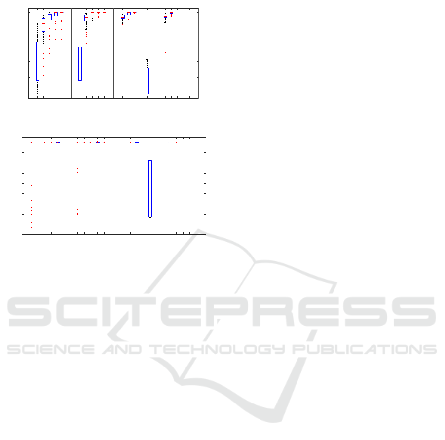
Each of the scenarios is set up 100 times and each

trial has a time limit of 3 minutes for the optimisation.

A summary of the runs is displayed in Fig. 7

First of all, it must be mentioned that the number

of feasible instances or instances for which a feasi-

ble solution was found within 3 minutes varies for the

different cases. While in the ﬁrst scenarios a feasi-

ble solution could still be found for almost all cases,

there are, for example, only 3 feasible solutions for

15 passengers and 6 trains. For three scenarios, no

feasible solutions were found or generated at all. In

some cases, it is also intuitive that there are fewer

VEHITS 2022 - 8th International Conference on Vehicle Technology and Intelligent Transport Systems

246

5 Pax 10 Pax 15 Pax 20 Pax

2T 3T 4T 5T 6T 2T 3T 4T 5T 6T 2T 3T 4T 5T 6T 2T 3T 4T 5T 6T

0.2

0.4

0.6

0.8

MIPGap

(a) Gap over different passenger (Pax) and train (T) sce-

narios.

5 Pax 10 Pax 15 Pax 20 Pax

2T 3T 4T 5T 6T 2T 3T 4T 5T 6T 2T 3T 4T 5T 6T 2T 3T 4T 5T 6T

100

120

140

160

180

Computation Time [s]

(b) Computation time over different passenger (Pax) and

train (T) scenarios.

Figure 7: Results for the computational study on the

Solingen–Wuppertal-Vohwinkel railway line.

feasible solutions. For example, it is more difﬁcult

to transport 15 passengers with 2 trains rather than

with 5 trains, especially if the requests are distributed

over the whole line. On the other hand, more trains

also create signiﬁcantly more conﬂicts, which lead to

greater complexity in ﬁnding a feasible solution and

are also more challenging to coordinate operationally.

In Fig. 7a the relative gap between primal and dual

solution of the optimisation problem (MIPGap) is de-

picted. To begin with, it can be observed that the gap

is always less than 1. This seems to indicate an under-

lying structure of the problem that the solver knows

to exploit. Furthermore, with the exception of one

outlier (15 passengers, 6 trains), it is evident that the

problem size is increasing and that better solutions

can be found more quickly for smaller scenarios.

Fig. 7b provides an insight on the actually used

computation time. Ignoring the outlier (15 passen-

gers, 6 trains) again, it can be observed that basically

only with the smallest train ﬂeet (2 trains) the compu-

tation took sometimes less than 3 minutes ﬁnding an

optimal or close to optimal solution.

The black-box pre-solving already indicates that

there seems to be potential for strong pre-processing

enabling the processing of larger instances. The de-

termination of the infeasibility of an instance is often

reached within the ﬁrst few seconds, which is crucial

because if the timeout were to occur without a solu-

tion, the situation with no solution and with a solution

not yet found would be indistinguishable.

5 CONCLUSION

Offering demand-responsive transport on rails can in-

crease the attractiveness, availability and accessibil-

ity of public transport, especially in rural areas. This

necessitates the efﬁcient use of resources, which re-

quires an optimisation of the activities involved. The

Integer Program presented in Sec. 3 models the prob-

lem with many facets.

Due to the time sensitive encoding of the vari-

ables, e.g. the dependence on time steps even in those

in which nothing happens the instance size grows very

fast. Correspondingly, the computation time is very

sensitive on the size of the time horizon. Some con-

straints, e.g. the enforced correct processing order in

Eq. (30)-(49), are not always necessary or even re-

dundant, but in some cases such as very large time

windows they are necessary.

All in all, the run time can possibly be de-

creased by either tuning black-box solvers such

Gurobi (Gurobi Optimization, 2020) for this task or

developing dedicated tailored algorithms such as by

Castillo et al. (Castillo et al., 2009). This approach

could then be supported by signiﬁcant pre-processing.

Another possibility is the development of heuristics

which provide (ideally provable) good solutions for

the problem. Besides the improvement of computa-

tion, the problem clearly demands for a robust formu-

lation which should be a logical next step. The vari-

ations in the requests over an extended period, e.g. a

year, should be considered as uncertain input and an

operator should be able to handle different scenarios.

The corresponding number of vehicles should be able

to satisfy the varying demand. Conclusively, the prob-

lem deserves a lot of attention and has much room for

improvement in various directions.

ACKNOWLEDGEMENTS

This work is funded by the Deutsche Forschungsge-

meinschaft (DFG, German Research Foundation) —

2236/1.

REFERENCES

Bisschop, J. (2006). AIMMS optimization modeling.

Demand-responsive Scheduling in Railway Transportation

247

Caimi, G., Kroon, L., and Liebchen, C. (2017). Models for

railway timetable optimization: Applicability and ap-

plications in practice. Journal of Rail Transport Plan-

ning & Management, 6(4):285–312.

Castillo, E., Gallego, I., Ure

na, J. M., and Coronado, J. M.

(2009). Timetabling optimization of a single railway

track line with sensitivity analysis. TOP, 17:256–287.

Castillo, E., Gallego, I., Ure

na, J. M., and Coronado, J. M.

(2011). Timetabling optimization of a mixed double-

and single-tracked railway network. Applied Mathe-

matical Modelling.

Cats, O. and Haverkamp, J. (2018a). Optimal infrastructure

capacity of automated on-demand rail-bound transit

systems. Transportation Research Part B: Method-

ological, 117:378–392.

Cats, O. and Haverkamp, J. (2018b). Strategic planning

and prospects of rail-bound demand responsive tran-

sit. Transportation Research Record, 2672:404–410.

Cordeau, J. F. and Laporte, G. (2003). The Dial-a-Ride

Problem (DARP): Variants, modeling issues and al-

gorithms. 4OR, 1:89–101.

Cordeau, J. F. and Laporte, G. (2007). The dial-a-ride prob-

lem: Models and algorithms. Annals of Operations

Research, 153:29–46.

European Commission (2020). Transforming europe’s rail

system.

Goossens, J.-W. (2004). Models and algorithms for railway

line planning problems.

Guan, D. J. (1998). Routing a vehicle of capacity greater

than one. Discrete Applied Mathematics, 81(1):41 –

57.

Gurobi Optimization (2020). Gurobi optimizer reference

manual.

Ho, S. C., Szeto, W. Y., Kuo, Y.-H., Leung, J. M. Y., Peter-

ing, M., and Tou, T. W. H. (2018). A survey of dial-a-

ride problems: Literature review and recent develop-

ments. Transportation Research Part B: Methodolog-

ical, 111:395–421.

Koch, T. (2005). Rapid mathematical programming.

Landex, A. (2009). Evaluation of railway networks with

single track operation using the uic 406 capacity

method. Networks and Spatial Economics, 9(1):7–23.

Li, F., Gao, Z., Li, K., and Wang, D. Z. (2013). Train routing

model and algorithm combined with train scheduling.

Journal of Transportation Engineering, 139:81–91.

Liebchen, C. and M

ohring, R. H. (2007). The modeling

power of the periodic event scheduling problem: rail-

way timetables—and beyond.

MATLAB (2020). version 9.7.0 (R2019b). The MathWorks

Inc.

Schindler, C. and von Stillfried, A. (2020). Fahren auf Sicht

- Ein Betriebskonzept f

ur den fahrerlosen Nahverkehr.

Eisenbahntechnische Rundschau, 69(10):22–27.

Schlaht, J., Frink, L., Laumen, P., Pfeifer, A., Schindler,

C., and Nießen, N. (2018). Automated Nano Trans-

port System - Ansatz zur Entwicklung autonomer

Schienenfahrzeuge. In Proceedings of the 1st Inter-

national Railway Symposium Aachen, pages 60–77.

Seraﬁni, P. and Ukovich, W. (1989). A mathematical model

for periodic scheduling problems. SIAM Journal on

Discrete Mathematics, 2:550–581.

Stein, D. M. (1978). Scheduling dial-a-ride transportation

systems. Transportation Science, 12:232–249.

Szpigel, B. (1973). Optimal train scheduling on a single

line railway.

Weik, N., Zieger, S., and Nießen, N. (2018). Trafﬁc

management heuristics for bidirectional segments on

double-track railway lines. In Operations Research

Proceedings 2017, pages 729–735. Springer.

VEHITS 2022 - 8th International Conference on Vehicle Technology and Intelligent Transport Systems

248