Suitability Analysis as a Recommendation System for Housing Search

Jaskaran Singh Puri and Pedro Cabral

NOVA Information Management School (NOVA IMS), Universidade Nova de Lisboa, Campus de Campolide,

1070-312 Lisbon, Portugal

Keywords: Suitability Analysis, Spatial Analysis, ArcGIS, GIS, Remote Sensing.

Abstract: The metropolitan cities are facing a huge skewness of service distribution that is given in different parts of

the same city. Given the rapid increase in immigration, the quality-of-life factors are often left out while

performing housing searches. This paper explores the ideal sub-regions in Delhi, India, for living based on

different lifestyle profiles. Using suitability analysis, it is possible to personalize a geographical area for

housing. Five such factors, namely, rental budget, commute time, green landscape, pollution, and food

accessibility were considered. Four different user profiles (18-65) and their importance to each of the factors

were simulated. The range of each variable was standardized using transformations. Data was obtained from

data-hubs like Kaggle, OSM, and GEE. The analysis was supported by ArcGIS Pro to get district-level

features and suitability modelling. The commute variable is a derived variable from the cost surface raster

and AQI values from the weather stations were used. Four different suitability maps are generated using multi-

criteria evaluation. This automated approach can be useful for customers and agents to find or consult housing

for immigrants by making it personalized and providing insights to better explain consumer behaviour based

on spatial attributes, hence making spatially intelligent tools.

1 INTRODUCTION

India, one of the fastest developing economies in the

world has a QoL (Quality of Life index) of 103 while

Switzerland maintains the highest QoL of 188 as per

Numbeo’s report of 2022. To add on, India faces the

burden of population and service centres to develop

for the people. Although with the advancement of

technology we (India) have been able to make major

improvements for the digital infrastructure and

collect enormous data, through spatial tools like

satellites or drones and aspatial tools like payment

systems, socio-economic surveys, or the generic tools

on the internet. However, with all the data we have,

we still struggle to address the QoL index which at its

root means improving housing indicators, crime rates,

and healthcare, among other statistics. We focus on

the very first indicator ie. housing and sustainability,

for eg, with some of the major Indian cities like Delhi,

Hyderabad, Bangalore, Chennai, Mumbai, and Pune

have become the major hubs for opportunities across

fields, it has also led to a huge inflow of people to just

a few of these cities. As a result, finding a sustainable

place to live in when moving to a different city for the

https://orcid.org/0000-0001-8622-6008

long term (Maclennan, 2012) has become of utmost

importance as it eventually will impact the country’s

QoL index. Most of the search tools that we use to

find accommodation on websites are generally

limited to budget and other accommodation

characteristics like area, beds, bathroom, WiFi, etc.

As a result of which, we often find ourselves looking

for better places to live in in the long run. It was

observed in a housing market study in London (Rae,

2016) that there exists a spatial mismatch between

search extent and housing characteristics which

explores an interesting result of what people are

searching for, in some cases, is likely to be found

outside their search extent.

A weighted suitability analysis to study the

growth of urban development was done by (Jain,

2007) for a city in India where variables like Land

Use and road accessibility are explored, as a result of

which the suitability maps matched with those of

urban expansion maps. Another suitability analysis

for educational land use using environmental was

done in Tehran by (Javadian, 2011) where factors like

access to schools, the slope of the area, and vicinity

to service centers were done. GIS-based studies

Puri, J. and Cabral, P.

Suitability Analysis as a Recommendation System for Housing Search.

DOI: 10.5220/0011014700003185

In Proceedings of the 8th International Conference on Geographical Information Systems Theory, Applications and Management (GISTAM 2022), pages 91-98

ISBN: 978-989-758-571-5; ISSN: 2184-500X

specifically for housing search (Xavier, 2012) were

also carried out. This study used classification as a

method to find the optimal value for the variables,

unfortunately, home-based variables like rental

pricing or dynamic variables like traffic changes were

not considered for this study. Moreover, the study

does not rely on user-weights hence not making

personalised decisions for the common people. A

house counselling study (Johnson, 2005) was also

carried out where the census data was used as the

primary source and was only intended for

organisations to provide counselling and provided

generic overall suitable areas-based house features.

This study aims to bridge the gap between aspatial

and spatial data, supported by GIS tools. It essentially

allows us to answer a simple question “What’s the

best place to do something?”. One such methodology

that enables us to perform this experiment is called

suitability analysis. The basic premise of which is to

help us find the best-suited decision based on some

requirements, rather than just giving the perfect

“solution/decision”.

One such critical advancement in the field of GIS

has been that of AHP or Analytical Hierarchy

Processes. AHP (Saaty, 2008) is an evaluation

procedure based on weighted qualitative and

quantitative factors. Majorly impacting site selection

and land suitability use cases across the industry.

(Bathrellos, 2017) was able to extend the core values

of AHP methodology to improve the urbanization

locations based on natural hazards and was able to

produce maps of suitable areas for development.

Due to the ever-changing landscape features of

any place, it was important for this study to consider

features that are generic to any place on earth. The

factors studied for this experiment capture both the

lifestyle aspects and age of a person, as also used by

(Sun, 2009) for land suitability in China. To carry out

a real-world simulation, we also assume four different

user profiles across the age range of 18-65. In our

experiment, we rely on ArcGIS Pro to carry out all

the important data transformation and

implementation of different algorithms.

This experiment will also address an important

hypothesis that “Spatial features do not affect the

lifestyle of an individual”. This can be observed in

our results by visualizing the different suitability

maps for the four user profiles. If we see similar

regions are recommended to all the users, irrespective

of their weights, that would mean we failed to reject

our hypothesis.

In the following section, the study area and its

related problems are discussed. Then the

methodology to experiment is presented. Finally,

results and relevant discussion is done for the various

simulations carried out for different users.

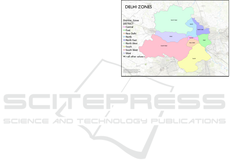
1.1 Study Area

Situated in the north-central part of India and on the

west bank of the Yamuna River, the capital of India,

Delhi due to its importance and rapid urbanization

was chosen as our study area, shown in Figure 1.

Figure 1: Map of Delhi, India is divided into 9 districts.

Spread over 1400 sqkm, Delhi, divide into 9 high-

level districts and further sub-divide into 32 divisions

as seen in Figure 1, is a highly populated area with a

population density of about 11,000 people per sqkm.

The landscape is mostly plain with over 33% of the

population residing in rental accommodation. The

city is one of the fastest-growing IT-hub in the

country and hence attracts millions of people to

migrate in the hope of a better future.

Delhi happens to be a good study area for our

experiment as it has a complex transportation system

of roads and metros that affects commute time and at

the same time is a great place for recreational

activities, work, and education. The city can support

people of almost all age groups as per their needs,

however, due to its large area, it can be hard to judge

as to what sub-region will suit a specific individual’s

needs.

2 METHODOLOGY

In this section, we will discuss the steps carried out to

execute this suitability analysis. It is important to first

set up a suitability modelling architecture that should

contain our goal and model criteria. The goal is the

outcome we would like to get from the model, as in

our case would be the top n divisions from the 32 that

suit a user’s lifestyle. On the other hand, criteria

GISTAM 2022 - 8th International Conference on Geographical Information Systems Theory, Applications and Management

would be the different factors that we are considering

as an input to the model. In our experiment, we’ve

decided on five such relevant factors rental budget,

commute time, green landscape, pollution, and

restaurant quality.

The reason for choosing these variables is to

enable a generic modelling scenario since the nature

of data presented here can be accessible for other

cities. With almost every country/city having a

dedicated website for housing search, food delivery

apps, weather monitoring platforms, the data for

rental budget, food accessibility and pollution is

accessible. On the other hand, the world-wide

coverage of Sentinel-2 and OSM-like data hubs will

allow free and open access to data for green landscape

and commute time calculation.

2.1 User Profiling

From a successful example of suitability analysis

(Albacete, 2012), where the experiment was being

simulated for multiple profiles, it was decided to

extend this approach for our experiment as well but

with an addition of user-specific weights. To run this

simulation for different users and test our hypothesis,

we created four different user profiles from the age

group 18-65 and their relevant weights or importance

for each of the five factors. The following table 1

shows the user profiling in detail.

Table 1: User Profiles with variables and weight

preferences.

Profile/ Age Variable Weight In %

A / 18

Commute Time 10

Rental Budget 60

Pollution 10

Green Landsca

e 5

Restaurant Qualit

B / 25

Commute Time 30

Rental Budget 10

Pollution 5

Green Landscape 5

Restaurant Qualit

C / 40

Commute Time 55

Rental Bud

et 5

Pollution 15

Green Landscape 15

Restaurant Quality 10

D / 65

Commute Time

Rental Budget

Pollution

Green Landscape 15

Restaurant Quality 1

2.2 Variable Definition

With the different variables that we have, the scale of

one form of data will rarely match the scale of other

variables. To address this, we use three different

transformation types small variable, large variable,

and user-specific variable.

Small Variable: When we have a negative

correlation between suitability and our variable i.e. if

the variable magnitude increases, the suitability

decreases.

 Rental Budget (RA): Scaled Range is 0 – 100

Formula Used: 100 – {input}

Example: If Input = 75, RA = 100 – 75 = 25

 Commute Time (CT): Scaled Range is 0 – 1

Formula Used: 1 – {input}

Example: If Input = 0.75, CT = 1 – 0.75 = 0.25

 Pollution (PL): Scaled Range is 0 – 1

Formula Used: 1 – {input}

Example: If Input = 0.25, RA = 1 – 0.25 = 0.75

Large Variable: When we have a positive

correlation between suitability and our variable i.e., if

the variable value increases, the suitability increases.

 Restaurant Quality (RQ): Range 0 – 5

Formula Used: {input} – 0

Example: If Input = 3, RQ = 3

User-Specific Variable: This is a special case when

we don’t want a variable to be on any of the extremes.

The ideal value is in the middle of a given range

 Green Landscape (GL): Range 0 – 1

Formula Used:

{input} > 0.5, 1 – {input}

{input} < 0.5, {input} – 0

Example: If Input = 0.6, GL = 0.4

2.3 Data Collection

Typically, a GIS application uses raster or vector

data, mostly obtained from satellites, drones, or

digitization of maps. The selection of data for this

study was based on their recency, accuracy, and

trusted open data providers.

For easier interpretation, we’ve divided the data

sources between Primary and Derived data. Primary

data refers to sources from which the data was used

as is, while derived data was extracted after a few

steps of processing.

Primary Data:

 Rental Budget data was acquired from Kaggle

which is a high-quality open data hub. Using the

Suitability Analysis as a Recommendation System for Housing Search

lat/long feature of this data it was possible to use

it for spatial analysis

 Pollution data was acquired from Central

Pollution Control Board for the AQI recorded

across different weather stations in the city

 Restaurant Quality data was also acquired from

Kaggle which consisted of all restaurants in the

city with their respective coordinates and food

ratings

 Green landscape data was acquired from Sentinel-

2A raster imagery obtained from Google Earth

Engine (GEE)

 The vector data for city-level districts, the road

network, and building polygons were obtained

from the OSM data-hub

 LULC map from ESRI 2020 was also used as an

input to distance analysis

Derived Data:

 Commute Time data wasn’t directly available in

the open hub. However, using OSM building

vector polygons, and LUCL map the traffic

intensity for each division was estimated

2.4 Data Preparation Structure

A summarized view has been displayed on the

previous page, Figure 2. for data preparation of our

project.

Figure 2: Showing a summarized view of how all variables

were prepared.

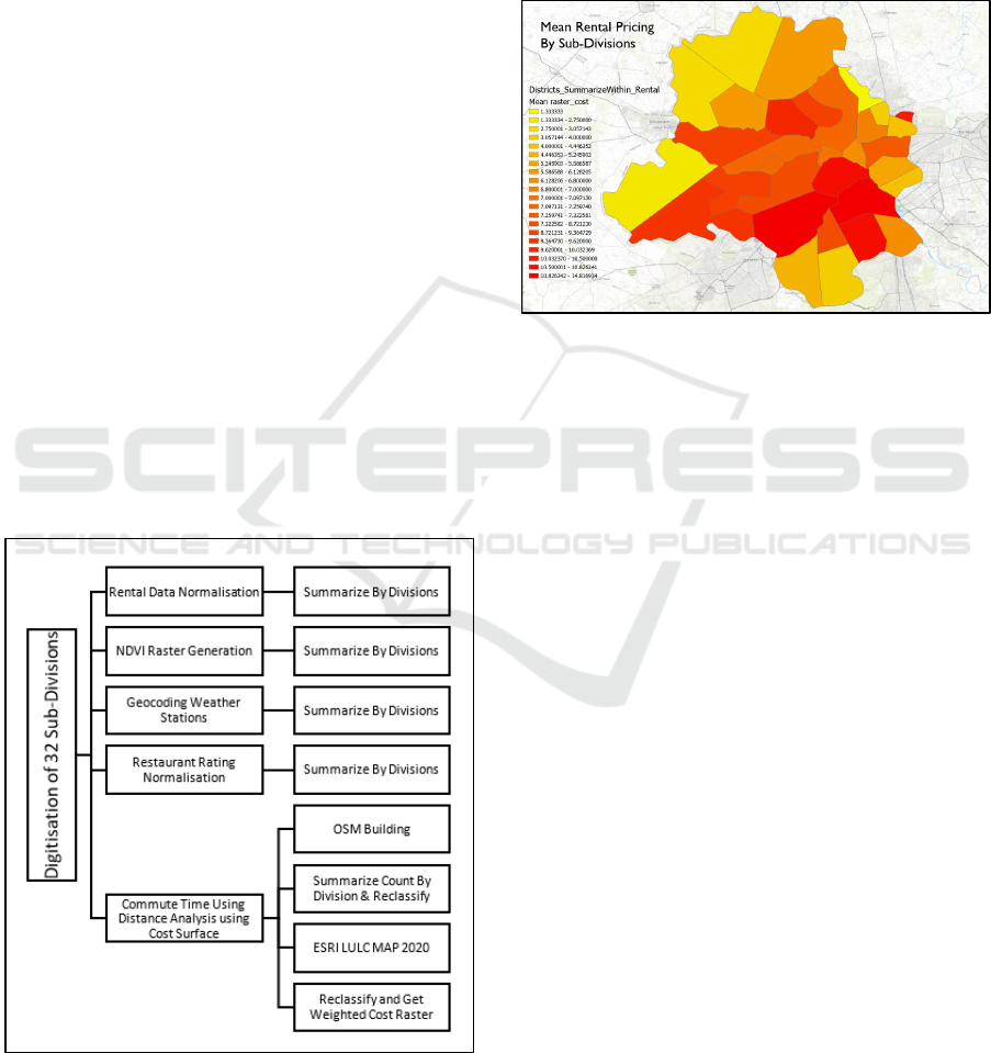
2.4.1 Rental Budget Variable

The accommodation budget is usually a very

important factor when choosing a new place to stay.

However, the pricing range can vary unevenly in

different areas of the city. Usually, rents are cheaper

in the outskirts of the city while it increases by a

factor of ‘x's as we move closer to the inner city.

Figure 3: Sub-divisions with mean rental pricing.

We observe a similar trend in the pricing of houses

across Delhi as shown in Figure 3.

As we can observe the dark red areas have higher

mean pricing of accommodations and the ones farther

away from the city are comparatively cheaper. For

this variable, we had a total of 17,790 rental points.

All the prices have been normalized between 0 to 1

and further on have been reclassified into 10 bins for

better standardization of data. Using the “Calculate

Field” option in ArcGIS Pro, a new field “raster_cost”

was created to store the reclassified values, finally

summarized by the division polygons using the mean

statistic.

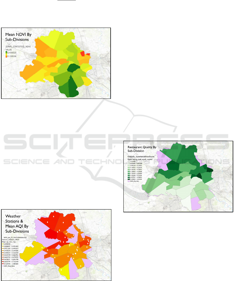
2.4.2 Green Landscape Variable

In modern cities, it is often hard to find such

landscapes especially due to the increase in

population and continuous deforestation. Greenery

has now become a luxury and has become an

important factor for the older age groups while

moving to a new place.

This kind of data is made available using raster

imagery of Sentinel-2A. Using the Google Earth

Engine (GEE) platform, which is a highly scalable

tool for geospatial analysis, the NDVI index was

calculated using our input shapefile of the entire city.

NDVI index is a mathematical combination of the

Red (B4) and NIR (B8) of Sentinel-2 to estimate the

amount of green density for a specific area. The

GISTAM 2022 - 8th International Conference on Geographical Information Systems Theory, Applications and Management

following formula was used for the calculation of this

index:

𝑵𝑫𝑽𝑰 

𝑩

𝟖

𝑩

𝟒

𝑩

𝟖

𝑩

𝟒

NDVI values for each of our 32 sub-division

polygons are shown in Figure 4.

Figure 4: Mean NDVI across sub-divisions.

2.4.3 Pollution Variable

The air quality index or AQI has now become an

important metric when evaluating the lifestyle of an

area, especially in developing countries where

urbanization is at its peak, the metro cities are the

highest impacted areas in the country. For our study

area, the AQI since the last few years has been

averaging between 300-400 which falls in the

“Severe” category.

For our study, we use 38 weather stations spread

across the city. Each station recorded its AQI values

as seen in Figure 5. To get division-level statistics

from station points, the addresses were geocoded

using ESRI’s Geocoding Database.

Figure 5: Locations of weather stations overlayed mean

AQI. Not all sub-divisions have AQI value.

2.4.4 Restaurant Quality Variable

Food accessibility and quality is yet another generic

assessment metric for realizing social life. This data

was initially collected from a local food delivery app

at a national level. Due to the raw nature of this data,

it was required to first clean the data for missing

values and normalization. Some restaurants did not

have any values for the delivery ratings and hence

were first imputed using spatial average i.e. for each

restaurant having missing values, they were imputed

with the mean of rating of restaurants in the proximity

of 10kms.

Further on, we had two rating variables initially,

food rating and delivery rating, both of which are on

a different scale. Another important factor was the

pricing of the food as well. Taking into account these

3 variables, the following variable with a custom

formula was developed:

𝑅𝑎𝑡𝑖𝑛𝑔  AVG(Food Rating + Delivery Rating)/Cost

Using this formula, whenever we have low pricing

for the food and a higher overall rating of food and

delivery, we get a higher value and vice-versa.

Finally, this new variable was scaled from 0 – 1. The

final result can be seen in Figure 6.

Figure 6: Sub-division level restaurant quality.

2.4.5 Commute Time Variable

Travel or commute time as other factors are yet

another important metric for our experiment. Due to

certain land types and urban development, some parts

of the city are the hardest to commute through. Traffic

data however isn’t something that is preserved by any

governmental or commercial organizations. The

following sources of data are explained in detail:

 OSM Data: Open Street Maps (India, North-East

Region 2021) provide us essentially the polygon

level data of various land types, as in our case

that’d be buildings and roads for our study area.

Suitability Analysis as a Recommendation System for Housing Search

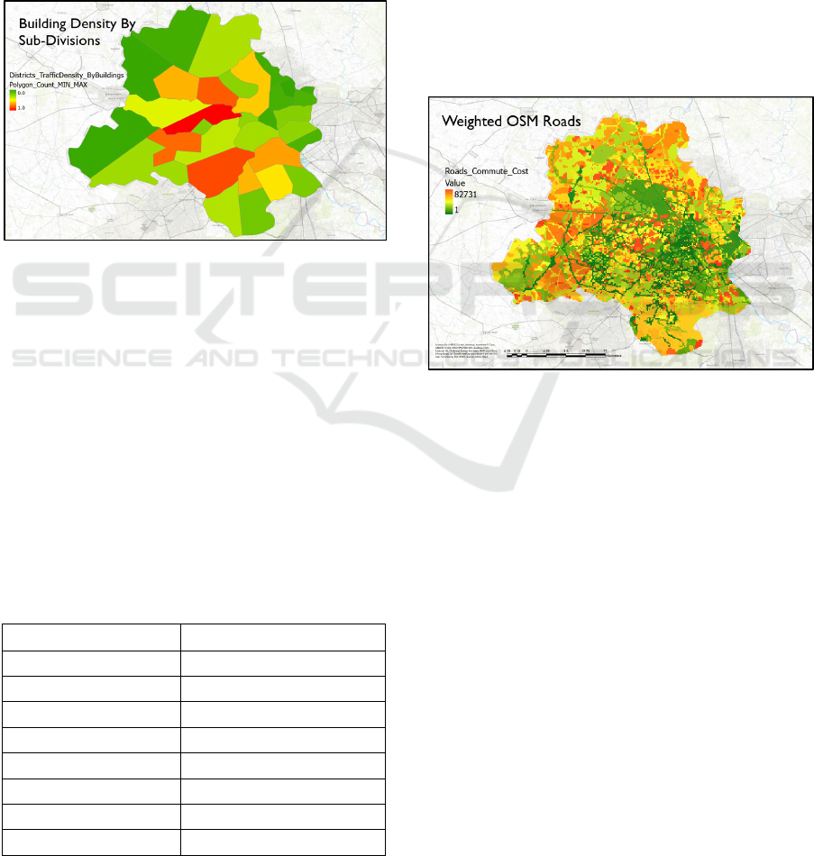
Using building polygons count we can assume

that a certain sub-division that has 0 buildings will

comparatively have minimum traffic congestion.

 LULC Data: The LULC map generated by ESRI

in 2020 for the entire globe. However, at a coarser

resolution, we still get an approximate idea if a

certain area is motorable or not. At a sub-division

level, this resolution of the raster image is enough.

The classes were reclassified to signify the

difficulty of the terrain type.

The following figures show the division level results

from the OSM data source, Figure 7.

Figure 7: Green divisions signify low building polygons

and red division shows a high cluster of buildings.

This data however does not represent any traffic or

commute difficulty over at a road level. It is neither

possible to say if, for example, it is harder nor easier

to travel from one polygon to another. To account for

this, we need data that is much more granular as

compared to a district level. As mentioned before,

LULC maps from ESRI combined with OSM road

maps can be used to infer such details. First, we re-

classify the land classes by their difficulty to

commute through. For example, the urban area is

easier to commute to than the water class. A complete

list of classes and their commute weights is

mentioned in Table 2.

Table 2: LULC and Commute Ranking.

Class Name Commute Complexity

Built Area 2

Shrub 3

Baren 3

Crops 4

Flooded Veg. 5

Grass 6

Tree 7

Water 8

To combine the two outputs, LULC commute map

and building density, a raster algebra operation was

performed with a 40% weightage given to LULC

maps due to low-resolution uncertainties, and 60%

weightage was given to the OSM based building

density. The following operation was done:

𝑅𝑎𝑠𝑡𝑒𝑟







0.4 𝑥 𝐿𝑈𝐿𝐶



  0.6 𝑥 𝐵𝑢𝑖𝑙𝑑𝑖𝑛𝑔





To obtain the cost of commute at a road level we used

the “Path Distance Allocation” tool from ArcGIS Pro

with OSM road maps and the weighted raster as

inputs. As a result of which the following output of

roads signifying their complexity to commute in

Figure 8 is shown. These values were however

summarised at a sub-district level to maintain

consistency across all variables.

Figure 8: OSM road network represented as a weighted

layer of commute toughness.

3 RESULTS AND VALIDATION

Once all the variables were prepared, we used ArcGIS

Pro’s in-built Suitability Modeller. Different

suitability analyses models for every profile were

built due to the change in weights for different

factors.

An important pattern that we can observe from the

four suitability maps is how the direction of

recommended locations starts to move towards the

south of the city as the weight of rental budget

variables starts to reduce. The inter and intra district

analysis of Delhi from 2011-2020 (M. Sharma, 2022)

also show similar spatial trends in terms of the quality

of life in the northern part of the city as compared to

the south. The liveable housing conditions that

include the availability of basic amenities are more

accessible in the northern sub-districts of the capital.

As per the reports, it was also observed that the north,

GISTAM 2022 - 8th International Conference on Geographical Information Systems Theory, Applications and Management

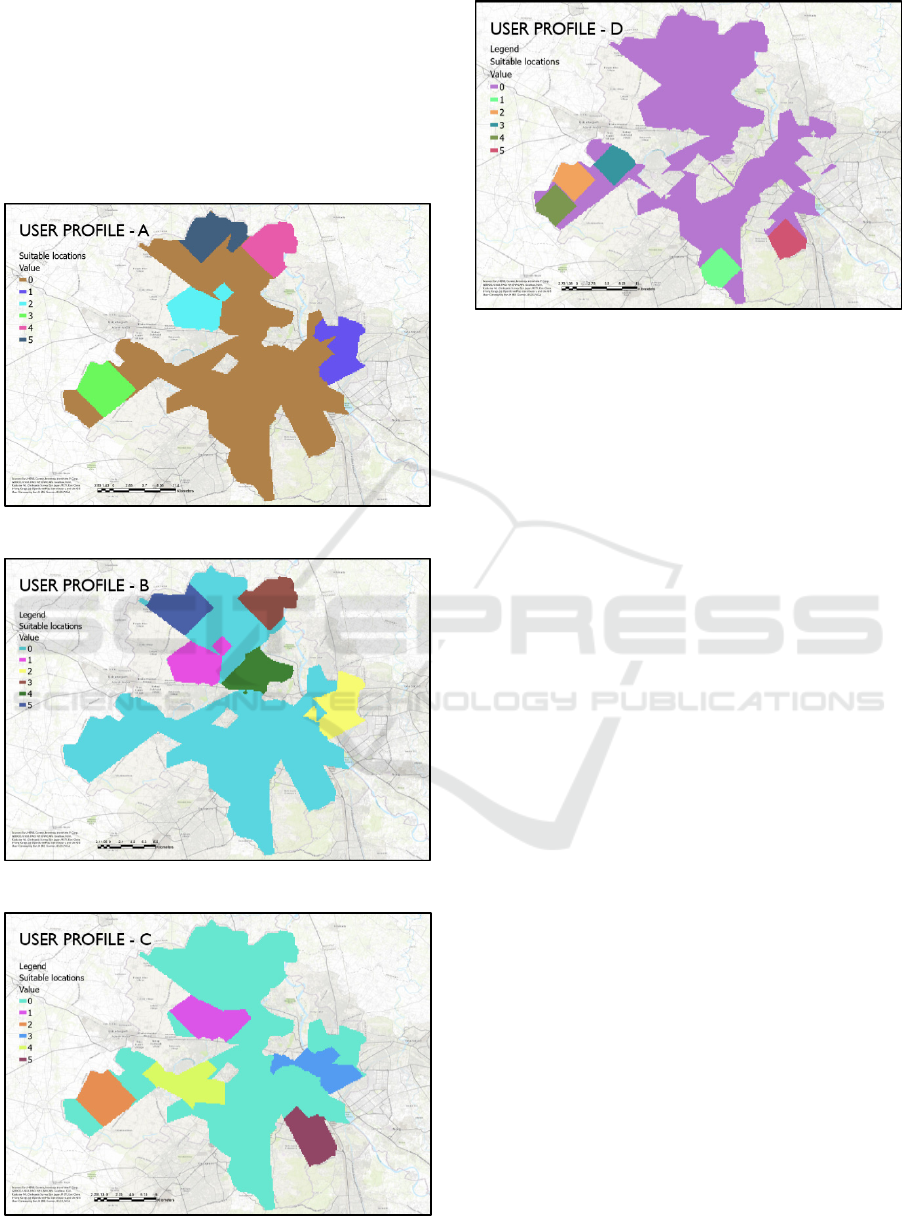
north-west, and central part of the city had the most

liveable housing conditions.

The southern districts, however, have a lower

percentage of liveable houses due to the difference in

the income-class groups, population density, and

patches of slums around these areas. The following

figures 9, 10, 11, and 12 show the most suitable

locations for the profiles A, B, C, and D to stay in.

Figure 9: Most suitable locations for Profile A.

Figure 10: Most suitable locations for Profile B.

Figure 11: Most suitable locations for Profile C.

Figure 12: Most suitable locations for Profile D.

4 CONCLUSIONS

In this study, we explored how suitability models can

also help us with social problems like finding the best

lifestyle-suited locations to live within a city.

Using GIS tools and methodologies, several data

points across five different variables were collected,

and by assuming a few user profiles we were able to

test our hypothesis that these variables play a vital

role in selecting optimal locations for different users.

GIS processing was supported by ArcGis Pro for

different geoprocessing tasks. However, a more

exhaustive analysis could have been done by bringing

in lifestyle variables from social media such as user-

interests per division through geotagged tweets or

other online data hubs, as done by (Zucca, 2008) by

including non-spatial data of social functions for their

suitability study.

As a limitation to the study, there is a presence of

geographical bias (as seen in the Modifiable Area

Unit Problem) in the study as most of the variables

are summarized to a broader geographical. This was

due to the lack of availability of data at a building

level. However, the need of using spatial tools for

real-estate and housing search platforms still

represents a strong use case for improving their

recommendation and search engines.

ACKNOWLEDGEMENTS

This study was supported by national funds through

FCT (Fundação para a Ciência e a Tecnologia) under

the project UIDB/04152/2020 - Centro de

Investigação em Gestão de Informação (MagIC).

Suitability Analysis as a Recommendation System for Housing Search

REFERENCES

Albacete, X., Pasanen, K., & Kolehmainen, M. (2012). A

GIS-based method for the selection of the location of

residence. Geo-Spatial Information Science, 15(1).

Bathrellos, G. D., Skilodimou, H. D., Chousianitis, K.,

Youssef, A. M., & Pradhan, B. (2017). Suitability

estimation for urban development using multi-hazard

assessment map. Science of The Total Environment,

575.

Jain, K., &. Y. V. S. (2007). Site Suitability Analysis for

Urban Development Using GIS. Journal of Applied

Sciences, 7(18).

Javadian, M., Shamskooshki, H., & Momeni, M. (2011).

Application of Sustainable Urban Development in

Environmental Suitability Analysis of Educational

Land Use by Using Ahp and Gis in Tehran. Procedia

Engineering, 21.

Johnson, M. P. (2005). Spatial decision support for assisted

housing mobility counseling. Decision Support

Systems, 41(1).

Rae, A., & Sener, E. (2016). How website users segment a

city: The geography of housing search in London.

Cities, 52.

Store, R., & Kangas, J. (2001). Integrating spatial multi-

criteria evaluation and expert knowledge for GIS-based

habitat suitability modelling. Landscape and Urban

Planning, 55(2).

Sun, J., Liu, Z., & Wei, Y. (2009, September). Spatial

Analysis and Present Situation Evaluation of Urban

Residential Land Suitability Based on GIS: A Case

Study in Changchun, China. 2009 International

Conference on Management and Service Science.

Zucca, A., Sharifi, A. M., & Fabbri, A. G. (2008).

Application of spatial multi-criteria analysis to site

selection for a local park: A case study in the Bergamo

Province, Italy. Journal of Environmental Management,

88(4).

Thomas L. Saaty (2005). Analytic Hierarchy Process.

Encyclopedia of Biostatistics.

Maclennan, D., & O’Sullivan, A.(2012). Housing Markets,

signals, and search. Journal of Property Research 29(4)

324-340.

M. Sharma, R. K. Abhay (2022). Urban growth and quality

of life: inter-district and intra-district analysis of housing

in NCT-Delhi, 2001–2011–2020”, GeoJournal, 1.

GISTAM 2022 - 8th International Conference on Geographical Information Systems Theory, Applications and Management