
Combining Deep Learning Model and Evolutionary Optimization for
Parameters Identification of NMR Signal
Ivan Ryzhikov
1
, Ekaterina Nikolskaya
2
and Yrjö Hiltunen
1,2
1
Department of Environmental Science, University of Eastern Finland, Yliopistonranta 1, 70210, Kuopio, Finland
2
Xamk Kuitulaboratorio, Savonlinna, Finland
Keywords: Evolutionary Algorithm, Deep Learning, Parameter Estimation, Artificial Neural Network, Predictive
Modeling, Nuclear Magnetic Resonance.
Abstract: In this study we combine deep learning predictive models and evolutionary optimization algorithm to solve
parameter identification problem. We consider parameter identification problem coming from nuclear
magnetic resonance signals. We use observation data of sludges and solving water content analysis problem.
The content of the liquid flow is the basis of production control of sludge dewatering in various industries.
Increasing control performance brings significant economic effect. Since we know the mathematical model
of the signal, we reduce content analysis problem to optimization problem and parameters estimation problem.
We investigate these approaches and propose a combined approach, which involves predictive models in
initial optimization alternative set generation. In numerical research we prove that proposed approach
outperforms separate optimization-based approach and predictive models. In examination part, we test
approach on signals that were not involved in predictive model learning or optimization algorithm parameters
tuning. In this study we utilized standard differential evolution algorithm and multi-layer perceptron.
1 INTRODUCTION
Time domain nuclear magnetic resonance method
(TD-NMR) is becoming highly attractive for
industries and meets various applications due to
relatively low price, mobility, easy operating, and
simple sample preparation procedure. The well-
known successful applications of TD-NMR
confirmed by international standards are solid fat
content determination in food and water (ISO 8292)
and oil content in oilseeds (ISO 10565). These
solutions are based on the difference of NMR
parameters of water and lipids and a low exchange
degree between these two fractions. There are studies,
which demonstrate applying the same approach for
analysis of lipid content in microalgae (Gao et al.,
2008) and for analysis of oil content of olive mill
wastes and municipal wastewater sludge (Willson et
al., 2010). Effects of flocculation on the bound water
in sludge measured by the NMR spectroscopy has
been studied in work (Carberry and Prestowitz,
1985).
Understanding the location of water molecules in
materials is important in process engineering because
it affects the dewatering process. Different situations
require different amount of energy for drying. The
other reason is the quantity of chemical components
to be added to the liquid to satisfy the desired
characteristics. Both factors take place in sludge
dewatering problem. Sludge is a semi-solid by-
product remaining after wastewater treatment. It is a
separated solid material suspended in a liquid,
characteristically comprising large quantities of
interstitial water between its solid particles (Global
Water Community, 2015). Typically, a polymer is
added to the wastewater to separate free water from
the solids, and it becomes easier to remove water
from the sludge. In wastewater treatment, the
dewatering of sludge is one of the most important
steps, because it affects largely both the process
economics and the costs of sludge disposal.
In sludges there are three water types, i.e. 1) free
water, 2) mechanically bound water, and 3)
physically or chemically bound water. The free water
can be easily removed by mechanical means, whereas
the bound water is held firmly within the floc, bound
to the sludge, or trapped between the sludge particles,
and thus cannot be easily removed (Jin et al., 2004).
The bound water can be further divided into
chemically or physically bound water, which is
Ryzhikov, I., Nikolskaya, E. and Hiltunen, Y.
Combining Deep Learning Model and Evolutionary Optimization for Parameters Identification of NMR Signal.
DOI: 10.5220/0011004200003122
In Proceedings of the 11th International Conference on Pattern Recognition Applications and Methods (ICPRAM 2022), pages 761-768
ISBN: 978-989-758-549-4; ISSN: 2184-4313
Copyright
c
2022 by SCITEPRESS – Science and Technology Publications, Lda. All rights reserved
761

removable only by thermal drying, and mechanically
bound water which is bound by weaker capillary
forces (Colin & Gazbar, 1995). It must be emphasized
that determining the water types is not
straightforward and based on the literature it is
difficult to reach an unambiguous interpretation on
the distribution of water within activated sludge
(Vaxelaire & Cézac, 2004). Furthermore, there seem
to be no studies focused on the analysis of water types
in sludge without a priori knowledge of the shares of
different water types.
To efficiently control complex sludge dewatering
process, we need to analyze the flow content to make
decisions on amount of heating energy and chemical
components to add. Analyzing the flow content
means solving the parameter identification problem.
NMR signals consist of a linear combination of one
or more exponential signals, which are traditionally
resolved by fitting them to an experimental signal.
However, in complex samples such as sludges, the
number and form of exponential signals are not
exactly known, making the analysis uncertain.
In this work, we start with the case when the
number of components is known. We use three
different approaches for system identification: the
first is based on parameters optimization via
evolutionary algorithms, the second is based on
parameters estimation via deep learning and the third
one is based on combination of evolutionary
optimization and deep learning prediction. We
numerically prove that proposed approach based on
combination of optimization and machine learning
outperforms baseline approaches: tuned optimization
algorithm and trained model.
2 REDUCTION TO
OPTIMIZATION PROBLEM
In this chapter we consider reduction of the water
content analysis to extremum seeking on the rational
vector space with constrains. Let us denote 𝑌 as
signal measurements, 𝑌=
𝑦
,𝑖=1,…,𝑛, 𝑦
∈𝑅,
and 𝑛 is the number of observations. Let us denote 𝑇
as times, where measurements 𝑌 were done, 𝑇=
𝑡
,𝑡
∈𝑅,𝑖=1,…,𝑛. In general case, we assume
that our measurements of signal are noisy, but in this
study, we start with assumptions that measurements
represent the real signal. The signal can be explained
by the following equation:
𝑦
(
𝑡,𝛼,𝜃,𝑐
)
=𝛼
𝑒
+𝑐
(1)
where 𝑚 is the number of components, 𝛼
are
amplitudes, 𝜃
are relaxation times and 𝑐 is
parameter. Now, using equation (1) we can formulate
the reduced problem:
𝐼
(
𝛼,𝜃,𝑐
)
=𝑦
−𝑦
(
𝑡,𝛼,𝜃,𝑐
)
,
(2)
𝛼
∗
,𝜃
∗
,𝑐
∗
=argmin𝐼
(
𝛼,𝜃,𝑐
)
,
(3)
where 𝛼
∗
,𝜃
∗
,𝑐
∗
are components amplitudes,
relaxation times and model constant, respectively.
We assume that we know the number of
components 𝑚, so to make water content analysis we
need to find solution on the vector space 𝑅
.
There is another criterion of our interest: the
accuracy in parameters. We cannot calculate this
criterion for the signal we observe, because we do not
know the real parameters, but it is possible in
simulation. Once we found solution of the problem
(2)-(3), it is possible to compare it to the real
parameters:
𝐼
(
𝛼,𝜃,𝑐
)
=
‖
𝛼
−𝛼
∗
‖
+
‖
𝜃
−𝜃
∗
‖
+
|
𝑐
−𝑐
∗
|
,
(4)
where 𝛼
, 𝜃
and 𝑐
are the parameters of the real
system (1) and
‖
∙
‖
is any norm on real vector space.
The major research question is if the solution of
problem (2)-(3) brings the extremum to criterion (4).
In experimental part we compare these criteria and in
the next section we describe the modifications of
criterion (2) that lead to performance improvement.
2.1 Adjusting Fitting Criterion
Our experiments proved that criterion adjustment is
one of the most important parts in increasing
performance of optimization and in this part, we
formulate the notations we use in the further study.
First, we modified the relaxation time variables
and use their exponential representation in search.
The reason for this is that amplitude and relaxation
time values are different in magnitude, 𝛼 takes values
approximately from interval
(
0,20
)
and 𝜃 takes
values from interval
(
0.004,0.04
)
. To equalize the
parameter values in search we use following
exponential transformation of relaxation times:
𝜃=
,
(5)
where 𝜃
is the variable we use in optimization.
ICPRAM 2022 - 11th International Conference on Pattern Recognition Applications and Methods
762

According to (2-3) and (5), the main criterion can be
formulated in the following way:
𝐼
𝛼,𝜃
,𝑐=𝑦
−𝑦𝑡,𝛼,
1
𝑒
,𝑐
,
(6)
𝛼
∗
,𝜃
∗
,𝑐
∗
=argmin𝐼
𝛼,
,𝑐
.
(7)
Criteria (2) and (6), as their minimum (3) and (7)
are identical but solving problem (6)-(7) is preferable
for some optimization algorithms.
Second, we add penalties for constrains violation.
We assume, that relaxation times and amplitudes are
bounded:
𝛼<𝛼
,𝜃
<𝜃
, 𝛼>0,𝜃
>0,
(8)
so the violation of constrains (8) will cause the
increase of fitting criteria (6):
𝐼
𝛼,𝜃
,𝑐=𝐼
𝛼,𝜃
,𝑐+𝛾
𝑃
𝛼,𝜃
+
𝛾
𝑃
𝛼,𝜃
,
(9)
where 𝛾
≥0 and 𝛾
≥0 are penalty coefficients,
𝑃
𝛼,𝜃
≥0 and 𝑃
𝛼,𝜃
≥0 are penalty function
of upper and lower boundaries, respectively:
𝑃
𝛼,𝜃
=
𝑓
(
𝛼
,𝛼
)
+
𝑓
𝜃
,𝜃
,
(10)
𝑃
𝛼,𝜃
=
𝑓
(
𝛼
,0
)
+
𝑓
𝜃
,0
.
(11)
In penalties (10) and (11), functions 𝑓
and 𝑓
are
linear functions of boundary violation:
𝑓
(
𝑥,𝑣
)
=
𝑥−𝑣,𝑥>𝑣
0
,
𝑥≤𝑣
,
(12)
𝑓
(
𝑥,𝑣
)
=
𝑣−𝑥,𝑥<𝑣
0
,
𝑥≥𝑣
.
(13)
By adjusting 𝛾
and 𝛾
parameters and penalties
(10)-(13) we can reach feasible and better solutions
of optimization problem (9). In experimental results
part we provide statistics that prove performance
improvement by adding penalties.
2.2 Generating Alternatives
Model (1) parameters have their boundaries, which
originate from the nature of identification problem
and expected components. Since we know these
values, we can generate alternatives according to
them. For example, when one utilizes stochastic
optimization algorithm, there is a need in initial
alternatives set. This is common in population-based
optimization.
First generating condition limits the amplitudes:
20> 𝛼
>0.1,𝑖=1,…,𝑚,
(14)
since in our experiments we study signals produced
by exponential additives, which amplitudes do not
exceed by 20.
Due to borders (14) we utilize uniform random
number generator, based on uniform distribution
𝑟
~𝑈
(
0.1,20
)
.
(15)
Generating of relaxation time is similar, but it
comes out of mixture of distributions
𝑟
~𝑈
(
0.01,0.06
)
,
𝑟
~𝑈
(
0.08,0.2
)
,
𝑟
~𝑈
(
0.03,0.06
)
,
(16)
and 𝑃
(
𝑟
=𝑟
)
=𝑃
(
𝑟
=𝑟
)
=𝑃
(
𝑟
=𝑟
)
=
.
Since the coefficient 𝑐 is expected to be small in
value, we also use a uniform distribution, where
density covers small interval around origin,
𝑟
~𝑈
(
−0.05,0.05
)
.
(17)
Each time we generate the initial population we
randomly generate alternative by generating variables
according to distributions (15)-(17).
2.3 Differential Evolution Algorithm
Optimization problem (2)-(3) is a global extremum
seeking problem on real vector field, as well as
optimization problem that includes penalties for
amplitudes and relaxation time parameters (14)-(15).
There are various algorithms for solving the problem
of this kind (Kochenderfer and Wheeler, 2019) and
speaking of global optimization the most of
algorithms are stochastic. And among stochastic
algorithms there are evolutionary algorithms and
bioinspired algorithms, which proved their
performance solving different challenging
optimization problems (Simon, 2013).
Today there are plenty of population-based
optimization algorithms and even more of their
Combining Deep Learning Model and Evolutionary Optimization for Parameters Identification of NMR Signal
763

modifications. It is impossible to examine each of
those for optimization problem and, perhaps, useless.
The only criteria we have is that if the algorithm of
our choice solves the problem with required accuracy
and in desired time. These criteria are related and
have different values for different computational
resources and are the subject of the further studies.
Since the problem aim is parameter identification
of specific system (1), we are not interested in
designing of general optimization algorithm, but
specific one, that has a high performance solving the
application problem. Reaching this aim requires two
steps. First, we need to prove that the reduced
optimization problem (2)-(3) or (6)-(7) is fitting
solving the component analysis problem (4). Second,
we need to examine one of the algorithms by varying
its parameters and determining a best one to have a
baseline approach, which we could use to compare
other algorithms in the future.
As a starting point for algorithms, we used
standard differential evolution (DE) algorithm (Storn
and Price, 1998). This algorithm has 4 control
parameters: mutation rate 𝑐
∈
0,1
, differential
weight 𝐹∈
0,2
, population size 𝑛
∈𝑁, and
number of iterations 𝑛
∈𝑁.
3 REDUCTION TO PREDICTIVE
MODELING
Machine learning approaches allows train the model
on data to recognizes the patterns. One of most
powerful approaches in a field of machine learning is
based on artificial neural networks (ANN). In this
study we utilize ANN, that takes the NMR signal as
an input and predicts the parameters of mathematical
model (1), that produced this signal.
Since we know the number of exponents in the
signal (1) and the distributions of mathematical model
parameters (15)-(17), we generated 𝑁=8∙10
of
parameters combinations and produced the same
number of signals (1). We also generated 𝑁
=
500 of parameters to test ANN model. Now, using 𝑁
observations of signal outputs and model parameters
that they produced we can train the ANN model and
then evaluate its performance on 𝑁
test
observations. Let us denote 𝑌
∈𝑅
,𝑖=1,…,𝑁, as
signals we use to train the model and 𝑌
∈𝑅
,𝑖=
1,…,𝑁
as signals we use to test it. Here 𝑅
is
vector field of size 𝑠=200, so ∀𝑖:
𝑇=
𝑡:𝑡 =0.04+ 0.02
𝑗
,
𝑗
=1,…,𝑠
,
𝑌
=𝑦:𝑦=𝑦𝑡
,𝛼
,𝜃
,𝑐
,
𝑗
=1,…,𝑠
(18)
The same 𝑁
observations will be used when
testing the proposed approach that combines ANN
predictions and DE algorithm search.
3.1 Data Preprocessing
Model (1) represents sum of inverse exponents, so
each signal observation contains a small number of
values greater than 1 and large number of values that
are very close to signal constant 𝑐.
First, we scale the all the signals (18) by
maximum observed value at each timestep 𝑗=
1,…,𝑠,
𝑌
=𝑦:
(
𝑌
)
max
(
𝑌
)
,
𝑗
=1,…,𝑠.
(19)
Second, we scale the outputs 𝛼
,𝜃
,𝑐
that
correspond to each of the 𝑖-th signal. For relaxation
times 𝜃
, we use min-max scaling, ∀𝑖,𝑗:
𝜃
=
(
𝜃
)
−min
(
(
𝜃
)
)
max
(
𝜃
)
−min
(
(
𝜃
)
)
.
(20)
For amplitudes and intercept parameters we
additionally scale them on signal maximum, ∀𝑖,𝑗:
(
𝛼
)
=
(
𝛼
∗
)
−min
(
(
𝛼
∗
)
)
max
(
𝛼
∗
)
−min
(
(
𝛼
∗
)
)
,
(21)
𝑐
̃
=
𝑐
∗
−min
(𝑐
∗
)
max
(
𝑐
∗
)
−min
(𝑐
∗
)
,
(22)
where ∀𝑖 : 𝛼
∗
=
(
)
and 𝑐
∗
=
(
)
are
scaled by maximum signal value amplitude and
intercept coefficient.
Proposed data preprocessing makes inputs and
outputs balanced. Predicted parameters can be
transformed to their initial form, by knowing the
signal characteristics and parameters involved in
(20)-(22) evaluations.
The same transformations (19)-(22) were applied
to test dataset, except for minimum and maximum
parameters, which were taken from the train dataset.
3.2 Artificial Neural Network Model
In this study we utilized multi-layer perceptron as
ANN structure. The structure of the model is given in
Table 1. At this stage of the research, we use a simple
architecture with rectified linear activation units and
do not apply regularization or dropout.
ICPRAM 2022 - 11th International Conference on Pattern Recognition Applications and Methods
764
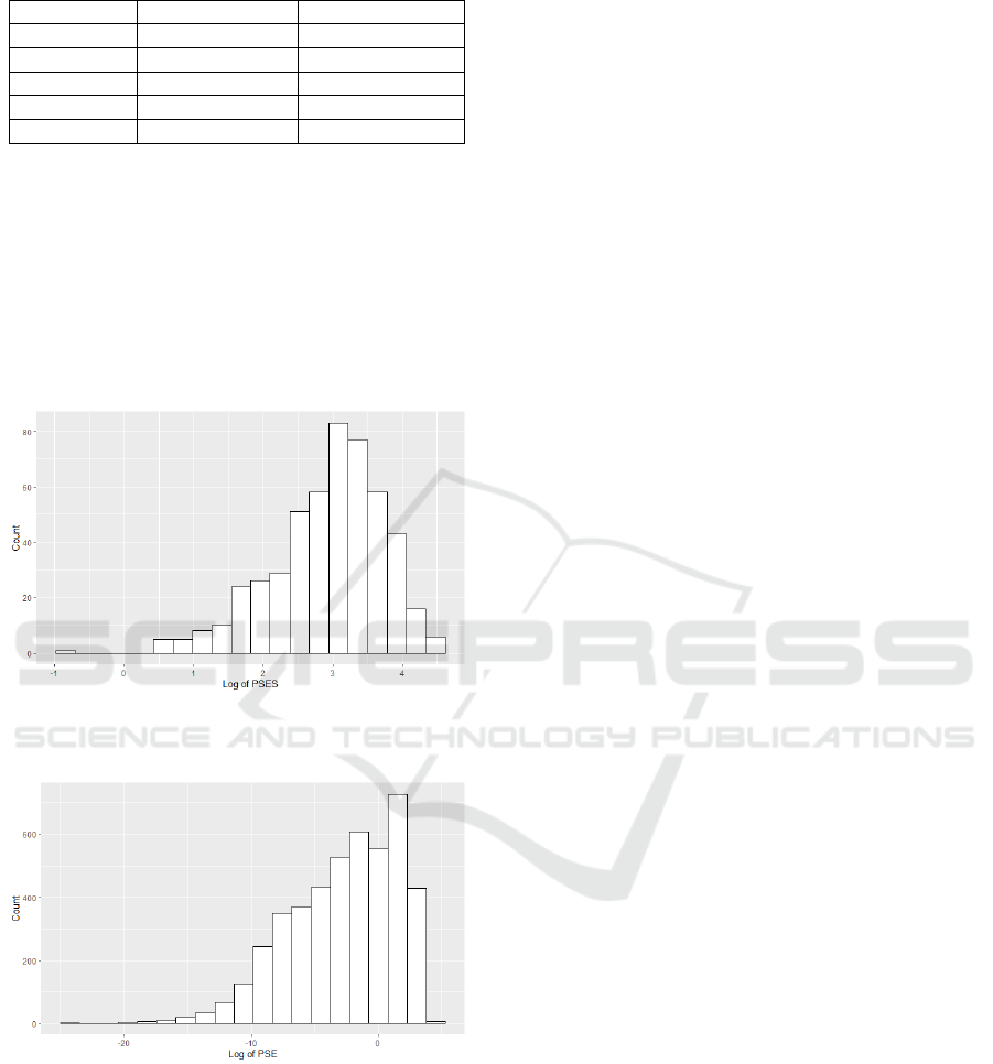
Table 1: The structure of ANN.
La
y
e
r
Activation Neurons
1 ReLU 256
2 ReLU 128
3 ReLU 64
4 ReLU 128
5 Linea
r
9
When training the model, we used 25% of train
dataset for validation. The training process stops
when the error on validation dataset begins to grow.
The histograms, showing the parameters square error
sum (PSES) is given in Figure 1. The PSES is in
logarithmic scale for better representation of the
parameter estimations error. The histogram showing
the distribution of parameter square error (PSE) for
each parameter prediction is given in Figure 2.
Figure 1: Histogram of PSES distribution for ANN-based
parameters predictor.
Figure 2: Histogram of PSE distribution for ANN-based
parameters predictor.
As one can see, the square sum of error is large.
That happens, because some parameters in the
prediction are predicted worse than others and their
squared value is large.
Histogram in Figure 2 shows that there are many
parameters which are predicted well and close to the
initial ones. Average error for amplitudes estimation
is 5.99, average error for relaxation times in
exponential form is 0.13 and average error of PSES is
24.52. Trained model with its characteristics will be
used as baseline model in the further studies.
4 PREDICTION MODEL IN
GENERATING INITIAL
POPULATION
Generating initial population for DE algorithm is
performed according to (15)-(17) random values
distributions. These distributions fit the real
parameters values boundaries.
The next step of our research is to combine ANN
models with optimization algorithm by generating
initial population partly according to distributions
(15)-(17) and partly by predictions of the machine
learning model.
Let 𝑎
,𝑖=1,…,𝑛
−1, be the alternative in
DE algorithm initial population, where 𝑛
<𝑛
is
the number of solutions generated on the basis of
ANN model prediction. Let the 𝑎
be an
alternative that is exactly the ANN model prediction
for the current signal input. Then for 𝑖=
1,…,𝑛
−1:
(
𝑎
)
=
𝑎
+𝑟,
(23)
where 𝑟~𝑁
(
0,𝜎
)
and 𝜎
is control parameter.
Generating initial population according to (23)
adds distorted ANN predictions and to the alternative
set and by controlling parameters 𝑛
and 𝜎
one
can tune the approach and find the best balance
between the randomly generated alternatives and
alternatives distributed normally around ANN
prediction of parameters.
5 EXPERIMENTAL RESULTS
First, we need to examine if the fitting criteria (2)
allows us to find the solution for the identification
problem (4). For that purpose, we run DE algorithm
for different combinations of its parameters: 𝑐
∈
0.01,0.05,0.1,0.2,…,0.9,0.95
, and 𝐹∈
0.1,0.2,…,2
. It is important to mention that each
run of optimization algorithm is done for the same
initial population, so different algorithm settings are
equal in their initial point. In this part of research, we
generated 20 of different initial populations that were
Combining Deep Learning Model and Evolutionary Optimization for Parameters Identification of NMR Signal
765
used by algorithm with each setting combination. For
each DE algorithm parameters and initial population
combination, we do 20 launches if different is not
mentioned. As a result, for each parameter
combination we have 20× 20=400 algorithm
runs. The idea of using the same initial population for
algorithm with different settings is explained in
(Jensen, 2013).
In this part of research, we would generate the
amplitudes in smaller area: from 0.1 to 1, instead of
20, as in (15). The initial signal was produced by the
following parameters of model (1):
𝛼
=
(
0.1,0.2,0.3,0.4
)
,
𝜃
=
(
0.004,0.01,0.018,0.035
)
,
𝑐
=0.
(24)
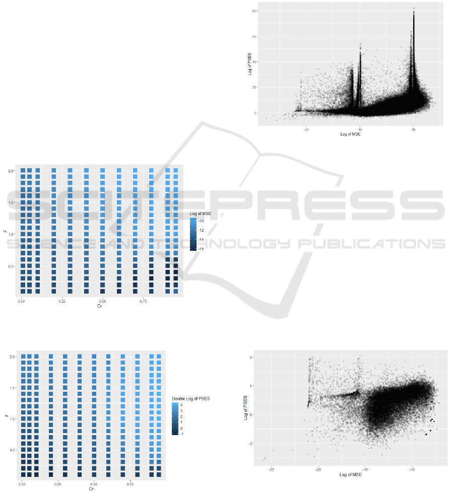
Let us start with criteria (2) without penalties,
population size of 100 and 500 iterations of
algorithm. The mean square error (MES) between
model and observations for different optimization
parameters is given in Figure 3. Similar plot but for
PSES criterion is given in Figure 4.
Figure 3: Influence of DE parameters on MSE. No
penalties. Number of iterations equals 500.
Figure 4: Influence of DE parameters on PSES. No
penalties. Number of iterations equals 500.
As one can see, different settings are better for
MSE and PSES criteria. But in real world we do not
know the real parameters and cannon calculate the
PSES criterion and, according to the results, we
cannot guarantee that improving of algorithm
performance for MSE criterion leads to better
parameters predictions.
Let us compare alternatives MSE and PSES
criteria on a scatter plot in Figure 5.
Figure 5: MSE vs PSES criteria for all solutions found by
DE with different parameters. No penalties. Number of
iterations equals 500.
Figure 5 shows that even though fitting criterion
has small values, parameter estimation can be far
from the real ones. There are many different peaks of
the PSES criterion, and those peaks are formed by
alternatives, which have too large 𝜃
parameters.
Since these parameters are in exponential form, these
exponents are becoming close to 0. In case of 0,
algorithm can find any amplitude as its multiplier and
that is why the criterion can have such a large value.
Also, there are other reasons for bad estimation of the
parameters, such as solutions with negative values.
But we know that these parameters cannot be too
large or negative, that is why we add penalties to the
Figure 6: MSE vs PSES criteria for all solutions found by
DE with different parameters. Criterion with penalties.
Number of iterations equals 500.
ICPRAM 2022 - 11th International Conference on Pattern Recognition Applications and Methods
766
fitting function and use criteria (6). The similar scatter
plot for fitting criterion with penalties is given in
Figure 6.
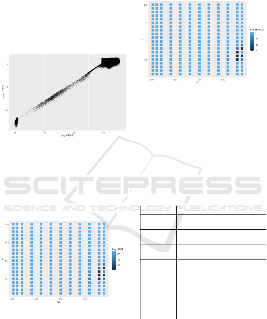
Our next step is to increase the computational
resources: we set the number of iterations to 7500
instead of 500. The scatter plot of MSE versus PSES
criterion is given in Figure 7.
Figure 7: MSE vs PSES criteria for all solutions found by
DE with different parameters. Criterion with penalties.
Number of iterations equals 7500.
Now we can see that there is a linear trend
between fitting and parameter estimation criteria and
can conclude that with these amounts of resources
algorithm finds good estimations when model fits the
observations. Heatmap for different DE parameters
influence on MSE is given in Figure 8 and their
influence on PSES in given in Figure 9.
Figure 8: Influence of DE parameters on MSE. Criterion
with penalties. Number of iterations equals 7500.
For this number of iterations, the best algorithm
parameters match both criteria. In the next part we
will use algorithm with 7500 iterations, 𝑐
=0.9 and
𝐹=0.6, as the best discovered algorithm settings.
Figure 9: Influence of DE parameters on PSES. Criterion
with penalties. Number of iterations equals 7500.
Now we examine algorithm on solving more
complex problem, where amplitudes can take values
from 0.1 to 20, as in (15). And for examination of
algorithm performance, we will use signals from
ANN training dataset.
We compared all three approaches in Table 2 by
different characteristics: criteria average and the
number of solutions that have logarithm of PSES
criteria smaller than 0, 1 and 2. We provided
Wilcoxon test, which p-value of 2.2𝑒
proves that
average of DE and DE+ANN algorithm is different.
Table 2: Characteristics of different approaches: ANN, DE
and DE+ANN.
Characteristic ANN DE DE+ANN
Average
PSES
24.52 63.37 39.12
Average log
of PSES
2.93 -2.57 -6.31
Average
MSE
5.65𝐸
1.04𝐸
𝟑.𝟏𝟐𝑬
𝟖
Average log
of MSE
-5.97 -31.46 -36.76
Log of PSES
< 0, number
1 80 128
Log of PSES
< 1, number
12 98 148
Log of PSES
< 2, number
69 131 189
Let us compare DE algorithm with DE algorithm
that involves ANN prediction in population
generating (23). Boxplot showing the difference in
MSE values between DE and DE+ANN algorithm is
given in Figure 10. Boxplot showing the difference in
PSES values is given in Figure 11.
Combining Deep Learning Model and Evolutionary Optimization for Parameters Identification of NMR Signal
767

Figure 10: Boxplot for logarithm of best alternatives MSE
values found by DE and DE+ANN approaches.
Figure 11: Boxplot for logarithm of best alternatives PSES
values found by DE and DE+ANN approaches.
According to Wilcoxon test, Figures 10-11, and
results in Table 2, we can conclude that combination
of ANN and DE outperforms other approaches.
6 CONCLUSIONS
In this study we examined three different approaches
for solving signal parameter identification by
observations. We applied evolutionary algorithm
with adjusted criterion, deep learning-based
approach, and a combination of those. We
numerically proved that fitting problem is related to
parameter identification problem. We trained a
baseline ANN model and optimization algorithm.
Numerical results proves that a combination of
DE and ANN for performing DE’s initial population
gives better results in solving signal parameter
recognition problem. Proposed approach outperforms
baseline approaches for different metrics, except for
average of parameter values error. This happens
because errors in its prediction are bigger than in
ANN’s but appears in fewer cases. The same proves
counting of PSES logarithm cases less than 0 or 1.
Further study is focused on designing deep
learning architectures and their combinations with
evolutionary algorithms that outperforms the
proposed approached and baseline approaches in this
study.
ACKNOWLEDGEMENTS
This research is a part of the Enerve projects, which
is funded by the Centre of Economic Development,
Transport and the Environment (ELY Centre) of
South Savo, Finland and four companies.
REFERENCES
Bower Carberry, J. and Prestowitz, R.A. (1985). Flocculation
Effects on Bound Water in Sludges as Measured by
Nuclear Magnetic Resonance Spectroscopy. Applied and
Environmental Microbiology, 49(2): pp. 365-369.
Colin, F. and Gazbar, S. (1995). Distribution of water in
sludges in relation to their mechanical dewatering. Water
Res, 29: pp. 2000-2005.
Gao, C., Xiong, W., Zhang, Y., Yuan, W. and Wu., Q.
(2008). Rapid quantitation of lipid in microalgae by time-
domain nuclear magnetic resonance. Journal of
Microbiological Methods, 75: pp. 437-440.
Global Water Community (2015). Sludge Drying Overview-
Treatment Methods and Applications. Available via:
http://www.iwawaterwiki.org/xwiki/bin/view/Articles/S
ludgeDryingOverviewTreatmentMethodsandApplicatio
ns
ISO 8292 (2008). Animal and vegetable fats and oils -
Determination of solid fat content by pulsed NMR.
ISO 10565 (1998). Oilseeds - Simultaneous determination of
oil and water contents - Method using pulsed nuclear
magnetic resonance spectrometry.
Jensen, T. (2013). Analyzing Evolutionary Algorithms.
Springer.
Jin, B., Wilén, B.-M. and Lant, P. (2004). Impacts of
morphological, physical and chemical properties of
sludge flocs on dewaterability of activated sludge.
Chemical Engineering Journal, 98: pp. 115-126.
Kochenderfer, M. J. and Wheeler, T. A. (2019). Algorithms
for optimization. MIT Press.
Simon, D. (2013). Evolutionary optimization algorithms.
Wiley.
Storn, R. and Price, K. (1998). Differential evolution - a
simple and efficient heuristic for global optimization
over continuous spaces. Journal of Global Optimization.
11 (4): pp. 341–359.
Vaxelaire, J. and Cézac, P. (2004). Moisture distribution in
activated sludges: a review. Water Res, 38: pp. 2215-
2230.
Willson, R.M., Wiesman, Z. and Brenner, A. (2010).
Analyzing alternative bio-waste feedstocks for potential
biodiesel production using time domain (TD)-NMR.
Waste Management, 30: pp. 1881-1888.
ICPRAM 2022 - 11th International Conference on Pattern Recognition Applications and Methods
768
