
Estimating Body Shapes from Measurements
Margarida Lima
a
, Joaquim Jorge
b
and Jo
˜
ao Pereira
c
INESC-ID Lisboa, Instituto Superior T
´
ecnico da Universidade de Lisboa, Av. Rovisco Pais, Lisbon, Portugal
Keywords:
Virtual Garment Fitting, Body Shape, PCA, Linear Transformation, Body Measurements.
Abstract:
e-Commerce now represents more than a third of apparel sales in the USA and accounts for most sales growth
year on year. However, it is still hard for people to buy clothes online because they have no idea how they
will look. Thus, we present an approach to model an approximation of a human body shape with a given
set of body measurements to fit virtual clothes. To estimate a new body shape from body measurements, we
developed two different models by using respectively linear transformations and PCA weights. Additionally,
we selected the minimum number of body measurements required to estimate a similar shape as the ground
truth. Finally, we evaluated our approach by comparing our results with estimations and visual evaluation
via pictures and measurements taken from real people. Results show that we can approximate human shape
through measurements with sufficient fidelity to simulate garment fitting.
1 INTRODUCTION
The percentage of online shopping increases year af-
ter year, and e-commerce captured an even greater
share of apparel sales throughout 2020 due to the
coronavirus pandemic with a leaps and bound growth
of 33.6%, to a total of $800 billion. The growth
pattern is expected to maintain reaching $908 bil-
lion in 2021 (Goldman, 2021). However, many still
prefer to buy clothes in physical stores instead of e-
commerce sites
1
One of the reasons relates to the
difficulty of modeling garments realistically and thus
hardly to know how a piece of clothing would look
when dressed (Pezzini, 2021). Most devices do not
have the resources to realistically simulate the fab-
ric’s physics, material, and texture. We approached
this problem by comparing two models, one only us-
ing linear transformations and the other using fea-
ture extraction, to see which is the best approach to
model a new body shape from only body measure-
ments. We also wanted to see whether using PCA
was helpful in mapping body shape with body mea-
surements. Therefore, we contributed by modeling
realistic 3D triangular meshes of human bodies, con-
sidering a set of body measurements that accurately
a
https://orcid.org/0000-0003-1762-8091
b
https://orcid.org/0000-0001-5441-4637
c
https://orcid.org/0000-0002-8120-7649
1
https://www.lsretail.com/resources/why-physical-
stores-are-still-vital-for-retail
output a polygon mesh with approximately the exact
measurements as the ones inserted by the user with
a similar body shape. We also defined the minimum
body measurements required to produce a mesh with
a similar body shape as the original one. Since our
target was virtual garment fitting, the produced body
shape needed to resemble the original one the clos-
est possible. Thus, the mesh quality evaluation was
performed by considering two criteria. The first one
consisted of comparing the final mesh directly with
the estimated one by measuring the distance between
the correspondent vertices of both meshes. Since we
did not scan people to validate our approach, we com-
pared the final mesh with silhouettes extracted from
pictures during the tests with real people. Thus, at
the testing phase, the users needed to manually insert
their body measurements and an RGB image of them-
selves wearing minimal or tight clothes. The second
criterion consisted of analyzing the final mesh mea-
surements and seeing how closely these matched the
original.
2 RELATED WORK
Until recently, body representation has been used al-
most entirely in the gaming industry to create realistic
characters. Amaury and Thalmann describe in (Aubel
and Thalmann, 2000) two major models to represent
the human body: surface models where a mesh only
318
Lima, M., Jorge, J. and Pereira, J.
Estimating Body Shapes from Measurements.
DOI: 10.5220/0011002900003124
In Proceedings of the 17th International Joint Conference on Computer Vision, Imaging and Computer Graphics Theory and Applications (VISIGRAPP 2022) - Volume 1: GRAPP, pages
318-325
ISBN: 978-989-758-555-5; ISSN: 2184-4321
Copyright
c
2022 by SCITEPRESS – Science and Technology Publications, Lda. All rights reserved

has skeleton and skin and multilayered techniques in-
cluding fat and muscle layers.
Surface Models. Most recent work done in creating
parametric avatars has been accomplished using ma-
chine learning techniques on a mesh database derived
from 3D scanned bodies of real people. After scan-
ning the necessary meshes, a system that estimates
body parameters can be trained. The usage of neu-
ral networks proved to be efficient in this topic. Re-
cent works PIFuHD (Saito et al., 2020) used neural
implicit functions for shape representation. In HS-
Nets (Dibra et al., 2016), the parameters themselves
are computed based on images as input, and are used
to reconstruct the 3D human shapes by using a statis-
tical human shape model based on SCAPE (Anguelov
et al., 2005). In HS-Nets, to learn the global mapping
from the data to the parameters, a convolutional neu-
ral network (CNN) is trained. This CNN is trained
by feeding the images from different views into the
network. However, providing a 3D mesh with this
system might lead to a wrong human body shape
representation by misleading its body measurements.
The same argument is applied to Detailed Human
Depth Network (DHDNet) (Zhang et al., 2020), where
Zhang uses CNNs in order to estimate a detailed and
completed depth map from a single RGB image that
contains occlusions of human body. Since informa-
tion is retrieved from an RGB image, there is no cer-
tain that the displayed body representation of the indi-
vidual in the image respects its body measurements.
After obtaining the desired parameters, we can esti-
mate a 3D model. The usage of blend shapes allows
an approach without requiring any machine learning
technique. Morphing requires a target shape to be
able to morph from the base shape until the desired
one. However, this kind of process requires a lot of
modeling work. One example is HMR (Kanazawa
et al., 2018), Zhang builds a standard model to be de-
formed and to recover occluded surface details using
the depth information. Both HMD (Zhu et al., 2019)
and Seo in (Seo and Magnenat-Thalmann, 2003) use
blend shapes to update the shape of a model in real
time by using an iterative interface. IntExMa (Volz
et al., 2007) uses a morphing algorithm to comply
with the desired body measurements as input. An-
other example is (Loper et al., 2015) where blend
shapes are used not only for body poses but also for
animations. SMPL (Loper et al., 2015) is a skinned
vertex based model that accurately represents a wide
variety of body shapes in natural human poses. This
project deforms a mesh according to its body pose us-
ing blend shapes, that were calculated through princi-
pal component analysis (PCA). Learning the human
body shape through PCA is a strategy used by a lot
of projects (Baek and Lee, 2012) (Anguelov et al.,
2005) (Loper et al., 2015) (Chen et al., 2019) and it
is an effective strategy to learn the variation between
different human body shapes, that is why this strategy
will be used in this proposal as well to learn the blend
shapes that most realistic modify a human 3D mesh.
Seo in (Seo and Magnenat-Thalmann, 2003), uses a
template mesh as using a database of 3D scanned
meshes from real people, and it is used as examples
to correspond a template mesh deformations with the
body measurements.
2.1 Multi-layered Models
Multi-layered Models. A multilayered model also
composed by some intermediary layers such as mus-
cle and fat layer which improves animation results.
This way, when the skeleton moves, that motion will
be reproduced by all layers with the skin reproducing
them all. Multi-layer Lattice (Iwamoto et al., 2015)
achieve that using voxels. With a mesh and muscle-
to-fat ratio as an input, this mechanism is able to fill
the interior and to get separated layers without any ex-
tra modeling work. Each voxel was classified accord-
ing to the muscle-to-fat ratio parameter that the user
inserted. The differentiation between layers is useful
for animation purposes, in which each layer behaves
differently. For instance, the fat should be much more
elastic than muscles. Another approach is to use pre-
vious modeled parts and adjust them to the inside of
the input mesh, like in Outside-In (Pratscher et al.,
2005). Similarly to Multi-layer Lattice, Outside-In
takes a mesh as fills the insides with artificial mus-
cles. Users can change muscle size in order to shape
avatars to taste.
3 OVERVIEW
Our development work was divided into three stages:
preprocessing, model generation, and evaluation. We
first repaired and segmented the samples in the pre-
processing phase before extracting the body measure-
ments. That was accomplished by using three dif-
ferent distances between points on the mesh: length,
height, and girth. The usage of geodesics was impor-
tant because it takes into account the mesh surface to
compute the distance. It simulates what a tailor would
do while measuring people. We then used that infor-
mation to build two models that estimate a new shape
based on a set of body measurements in the model
generation stage. The first one used feature extraction
to learn the principal components that vary in a human
body, and the second directly mapped body measure-
Estimating Body Shapes from Measurements
319

ments with coordinates using linear transformations.
Finally, we validated the results obtained according to
the shape and body measurements using both samples
from the dataset and tested with real people.
3.1 Preprocessing
The input meshes were delivered by the Semantic
Parametric Reshaping of Human Body Models (Yang
et al., 2014), a dataset with 3000 meshes, where 1500
are male and 1500 are female. Each mesh contains
12500 vertices and all meshes are positioned in a
neutral pose. All samples have been placed in point
to point correspondence, means that for two meshes
m
1
and m
2
all vertices v
i
∀i in V are in the same
semantic region. We use this dataset to extract the
coordinates of each samples as well as their body
measurements. We used manual segmentation in a
single mesh using Blender interface
2
, and replicate
it to the other meshes using a Python and Blender
integration module - blenderpy
3
. This is possible
due the point-to-point correspondence on the dataset.
Mesh Repair. The results of (Yang et al., 2014)
assume all meshes do not contain any non-manifold
vertices. However, a preliminary analysis using
Blender led us to conclude that most meshed con-
tained non-manifold vertices which could interfere
with extracting body measurements. We fixed these
problems using Wrap 3, a professional tool developed
by Russian 3D Scanner
4
.
Body Measurements. Users manually inserted body
measurements as the system’s input. The measure-
ments required were split into three different cate-
gories: girth that measures the distance around the
middle of something, length and height that measure
the distance between two points. While lengths are
measured on the mesh surface heights are not. The
point correspondence property of the dataset is use-
ful once more to extract the body measurements, we
manually selected the initial and target points used
to measure in one sample of the dataset and repli-
cated it to the remaining meshes. Height measures
the distance between two points using the Euclidean
Distance on the z axis (the vertical one). The length
measures the distance between two points considering
the mesh’s surface that contains the initial and target
points. For this measurements we used the geodesic
distance. We calculate a geodesic using a modified
Dijkstra search algorithm (Dijkstra, 1959) to find the
2
https://www.blender.org/
3
https://pypi.org/project/bpy/
4
https://www.russian3dscanner.com/
shortest paths between vertices. Differently from Di-
jkstra, geodesics can intersect edges to form straight-
line paths. Last, we compute girth measurements by
intersecting a plane with the mesh.
3.2 Model Generation
We compared two distinct methodologies against
each other. The first uses linear transformations to
output a new body shape, while the second applies
feature extraction to explain the maximum variance
in the human body. But first, we performed unsu-
pervised feature selection on the original dataset
to obtain the minimum measurement subset that
accounted for as much information as possible.
Since there was no a priori classification of shapes,
supervised methodologies for body measurement
selection were ineffective. Feature selection reduced
characteristics to approximately 17%, down to seven
features from the initial 41. Both of our models used
the subset returned from the feature selection process
to output new body shapes.
Feature Selection. Unsupervised Feature Selection
consisted on analyzing the dataset to filter 34 mea-
surements out of 41. We proceeded to the distribution
analysis of each variable. We replaced all outliers
that were outside of the µ ± 3σ Gaussian boundary
by missing values, to prevent entropy in our system.
The missing values count after replacing the outliers
indicated that girth measurements were more affected
by missing values than the other measurements,
specially the underbust girth, bicep girth, armhole
girth and knee girth. Since those measurements were
prone to high amounts of error, we decided to exclude
them from the final subset. Next, we normalized all
variables, sorted them by variance and selected the
ten variables that vary the most, resulting in the mea-
Table 1: Top 10 body measurements subset per gender
sorted by higher (1) to lower (7) variance. Both subsets
have 6 elements in common, but with a different variance
level. BM stands for body measurement.
BM
Gender
Male Female
1 Bust Girth Bust Girth
2 Hip Girth Hip Girth
3 Thigh Girth Abdomen Girth
4 Rise Length Thigh Girth
5 Waist Girth Height
6 Abdomen Girth Waist Girth
7 Height Mid-Thigh Girth
8 Underbust-to-Belly-
Button Length
Waist Height
9 Neck Girth Inseam Height
10 Waist Height Hip-to-Ankle Height
GRAPP 2022 - 17th International Conference on Computer Graphics Theory and Applications
320

surements represented in Table 1. Next we calculated
the correlation between the top 10 measurements and
concluded that all height measurements are highly
correlated. Thus, besides height, any other height
measurement in the top ten could be removed without
losing information loss. By only maintaining the
height measurement from the top ten measurements,
the female subset resulted with seven measurements
and the male one with nine. In the male dataset, the
neck girth is correlated with the rise and underbust to
belly button lengths and we only maintained the neck
girth measurement. We ended up with two subsets
of seven body measurements, as shown in Table 2
with a highly uncorrelated variation. Both subsets
shared six measurements, leaving only one unique
measurement for each gender: neck girth for males
and mid-thigh girth for females. We thus reduced the
initial dataset by almost 83%.
Estimating Body Shapes with PCA The feature se-
lection was applied on the dataset containing the body
measurements, while the feature extraction was per-
formed on the coordinates dataset. The feature extrac-
tion was performed on the coordinates dataset using
Principal Component Analysis (PCA). We first calcu-
lated the template meshes for each gender, that are
the mean of all samples. We then followed a sim-
ilar approach to Wuhrer proposal for estimating hu-
man shapes based of body measurements (Wuhrer and
Shu, 2012). As input to the method, it was given a
database of n triangular manifold shapes S
0
,..., S
n−1
of
human bodies with similar posture and a set of mea-
surements M. Let M
i
denote the measurements corre-
sponding to S
i
. Our aim is to estimate a shape S
new
that interpolates the distances M
new
. This approach
proceeded by learning the correlation between the
shapes and the measurements. The template meshes
¯
S were used to calculate how much the samples dif-
fer from the average shape. Therefore, there is a new
dataset D that is composed by the differences between
all shapes of S and
¯
S. Let D be a (3v × n) matrix. We
performed PCA in D, and it yielded a matrix W that
Table 2: Final body measurements subset per gender sorted
by higher (1) to lower (7) variance. Both subsets have the
first 6 elements in common (even with a different sequence)
and only the last element of both subsets is unique.
BM
Gender
Male Female
1 Bust Girth Bust Girth
2 Hips Girth Hips Girth
3 Thigh Girth Abdomen Girth
4 Waist Girth Thigh Girth
5 Abdomen Girth Height
6 Height Waist Girth
7 Neck Girth Mid-Thigh Girth
corresponded to the transformed dataset D. The ma-
trix W and matrix D are the representation of the same
information but in different spaces. By applying PCA
to D we extracted the information in the dataset by
creating a new coordinates system that fitted the data
where it varies the most. We lost information regard-
ing the variables of D because new ones were created.
However, if D and W are the same matrix in different
coordinates systems, there was some matrix A that de-
fines the transformation between them. Thus, a new
shape S
new
can be estimated via Equation 1 where the
sum of the template mesh
¯
S and the weights of a new
set of measurements W
new
transformed by A yields
S
new
.
X
new
= AW
new
+ µ (1)
However we still needed to calculate matrices A
and W
new
. We knew that W is D transformed into the
PCA coordinate system, thus A is responsible for the
coordinate system swapping. So we can infer A from
D and W, according to Equation 2 with D
+
being the
pseudo-inverse of D.
W = AD ⇔ A = W D
+
(2)
To calculate the weights matrix W
new
, we took into
consideration the body measurements and the PCA
weights W
i
of each shape S
i
. For that, we learned a
linear mapping from M
i
to W
i
with i = 0, ..., n − 1,
by transforming each M
i
to a new coordinate system
W
i
. To perform this, we calculated another transfor-
mation matrix B that maps body measurements to its
corresponding PCA weights, as shown in Equation 3,
where M
+
is the pseudo-inverse of B.
W = BM ⇔ B = W M
+
(3)
With this, we were able to relate the body mea-
surements to the information extracted from the hu-
man body variation through PCA and give it a weight.
To reproduce the results obtained in (Wuhrer and Shu,
2012) we normalized each entry of W by its corre-
spondent PCA eigenvalue. Finally, to estimate a new
shape X
new
based on a new set of body measurements
M
new
, we transformed M
new
to the PCA coordinates,
that resulted in a weight vector W
new
and then trans-
formed W
new
to the coordinate system that dictates the
shapes. Therefore, we rewrote the Equation 1 into
Equation 4.
X
new
= ABM
new
+ µ (4)
The mapping between the measurements and the
PCA weights of the 3D shapes allowed us to find
an new shape S
new
given a new set of measurements
M
new
. With this process we understood how much the
human shape vary from the average human shape
¯
S.
We related that variation with the body measurements
M and estimate new shapes S
new
with a new set of
Estimating Body Shapes from Measurements
321
body measurements M
new
. By adding the weights cor-
responding to a new set of body measurements W
new
to the template mesh
¯
S we obtained a new shape that
respects the variation dictated by M
new
.
3.2.1 Body Shape from Linear Transforms
Body Shape from Linear Transforms. In this
model, a shape can be directly obtained from the body
measurements. We accomplished this by creating a
transformation matrix between the coordinates and
body measurements datasets. Let us use the same ma-
trices and variables as in the previous model and as-
sume that there is a function T that maps a measure-
ments vector M into a vector of vertices coordinates S.
In this case, A represents a linear transformation map-
ping the space of body measurements to the space of
3D coordinates, as represented as in Equation 5.
S
new
= AM
new
(5)
Notice that S
new
returns a column vector with 3v ele-
ments, therefore A was a (3v × m) matrix. Also note
that A had 3v rows and m columns, whereas the trans-
formation was from ℜ
m
to ℜ
3v
. To calculate the trans-
formation matrix A we needed to start from Equation
5 and isolate A, just as demonstrated in Equation 6.
S = AM ⇔ A = SM
+
(6)
4 EXPERIMENTAL EVALUATION
We divided the evaluation into validation and evalua-
tion processes. The validation was intended to verify
if models were performing as expected. We observed
which model performed the best and used the winner
to the final evaluation process that involved real
users. Both processes were evaluated regarding the
shape and measurements of the estimated results.
4.1 Validation
To validate both models, we selected four different
samples from the database. These included two male
and two female scans, one smaller and the other
larger. Using samples that cover many variations
of human shape is essential to see whether the
techniques can deal with comprehensive cases.
Body Shape. We calculated the distance between
the correspondent vertices of the ground truth
samples and the estimated ones. With all distances
calculated, we visualized the error using a color
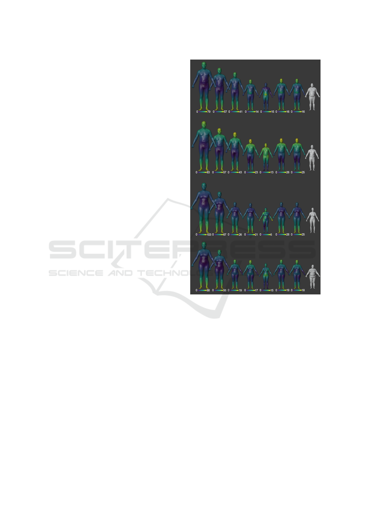
Figure 1: PCA Error color map using different measure-
ment sets. Each column corresponds to a subset of the top
ten body measurements or from the selected seven from Ta-
ble 2, from left to right: (a) top two (b) top four (c) top six
(d) top eight (e) top ten (f) selected six (g) selected seven (h)
original shape. The yellow parts denote higher error, while
the areas in dark blue are closer to the original shape.
map, like represented in Figures 2 and 1. Each
column represents a different subset, from right to
left: top 2, top 4, top 6 , top 8, top 10, selected 6,
selected 7 and ground truth. We estimated the same
shape using the seven different body measurement
subsets. To address to a specific estimation we use
the nomenclature (xy) where x is the row number and
y the column. We saw that the results were often
better when using more measurements. This was
supported by the MSE values, since they were higher
as the number of measurements used to estimate a
new shape decreases. However, in Figure 2 we saw
that the difference between (1d) and (1e) is almost
0 and their MSE difference was about 0.0002. This
GRAPP 2022 - 17th International Conference on Computer Graphics Theory and Applications
322
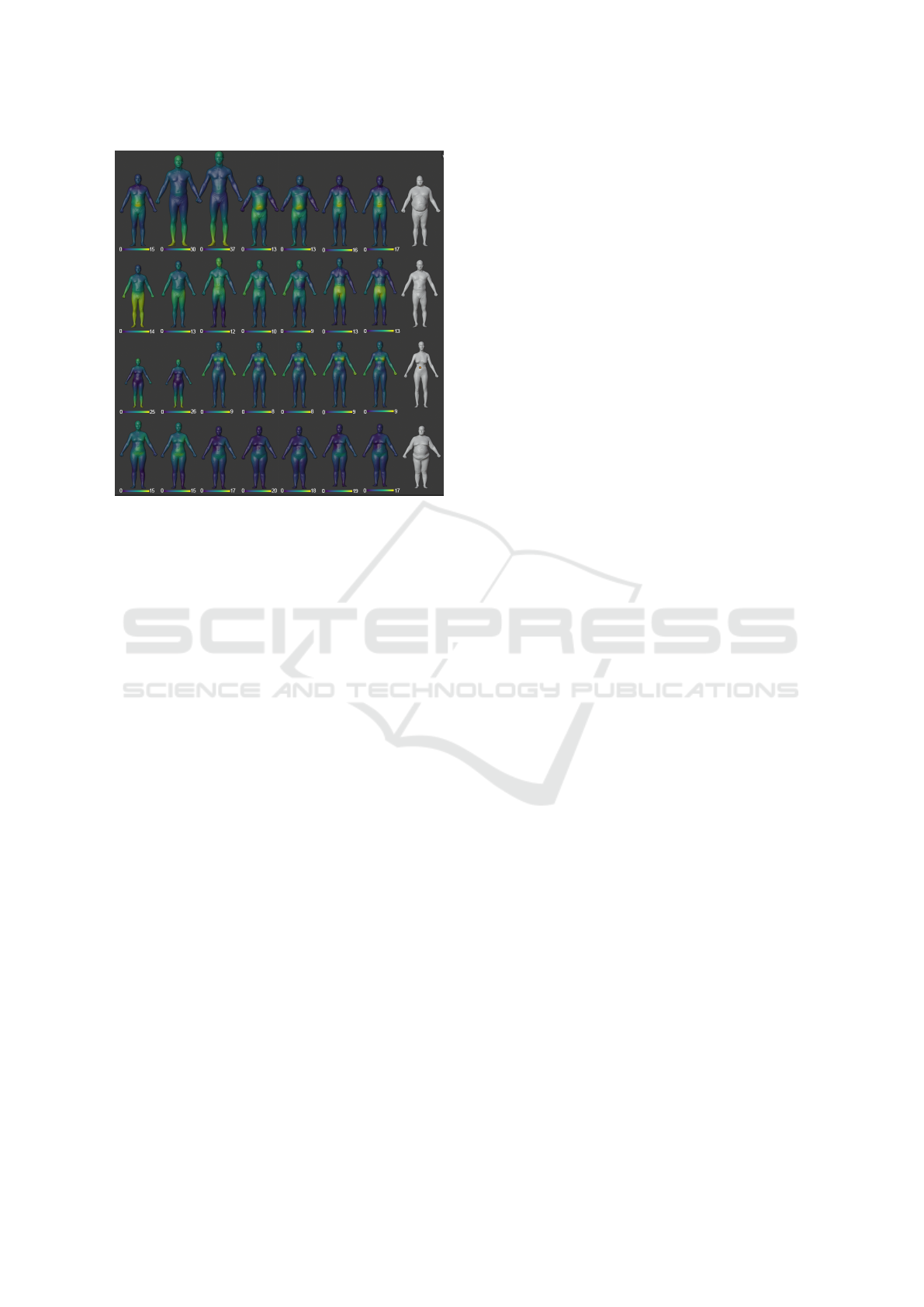
Figure 2: Linear Model Error color map with different mea-
surements set. Each column corresponds to a subset of the
top ten body measurements or from the selected seven from
Table 2, from left to right: (a) top two (b) top four (c) top
six (d) top eight (e) top ten (f) selected six (g) selected seven
(h) original shape. The yellow parts have a higher distance
error, while the dark blue parts are closer to the original
shape.
indicates that the insertion of the body measurements
nine and ten is irrelevant, and that we can obtain the
same results using only the first eight measurements.
In (1c) of Figure 2 we noticed a big difference in the
height comparing the original sample. This happened
specially to male meshes because the height is not
part of the top six measurements, however it is
more noticeable in (1c) than in (2c). This happened
because of the high values of the remaining measure-
ments, like waist bust, abdomen, etc. Like sample
SPRING306’s body measurements were way higher
than average on the dataset and there were not many
samples with bigger sizes, the model estimated a new
shape using the information that it had. This resulted
in a shape that was very similar to the average male
body, but in a bigger scale. This explained why
in (1b) and (1c) of Figure 1 had a higher distance
difference of sample SPRING0306 in their feet and
head, since the center of all meshes is on their groin.
To produce a shape with such big measurements,
the model scaled the shape in order to respect them
and the model ends up being huge because in top six
measurements we do not have height as a constraint.
This effect is also visible in (1b) regarding the top
four measurements, however in (1a) it is not visible.
It is visible that in (1a), (1b) and (1c) the main
differences regarding the original mesh are in the
belly. Sample (1g) was characterized by having larger
dimensions and our linear model had difficulties rep-
resenting those dimensions to perfection. However
it returned a shape with larger dimensions but not
as big as the ones inserted. This happened because
groups of male with larger dimensions were poorly
represented in the Semantic Parametric Reshaping
of Human Body Models dataset (Yang et al., 2014).
The estimation presented in (1a) was very similar to
those in columns (1d) and (1e). While its maximum
error was similar(15cm), it failed to represent the
belly more similarly. We expected the columns (1g)
and (1g) to perform better since the subsets were
composed by body measurements that were obtained
through feature selection, represented in Table 2.
However, missing measures such as height and
underbust-to-belly button hurt the returned shape,
especially on the belly of the estimations where they
had a higher distance error. Analyzing the estimation
of sample SPRING0306 and its MSE values, we
concluded that the best subset of body measurements
is the top eight.
Body Measurements. We validated the body mea-
surements extracted from the estimated shapes with
the original ones. The body measurement extraction
of the estimated shapes was made just like the extrac-
tion of the measurements of the original shape was
made. We observed that our linear model was more
able to estimate shapes that belong to a group that is
well represented in the dataset than samples that are
poorly represented. Which means that the estimated
measurements of average shapes were more similar to
the original ones. In one of the female estimations we
observed that all subsets, except for top four and top
two, performed relatively well with a bigger error rate
on the girth measurements. Thus, since the subsets
obtained from Table 2 did not produce better results,
we discarded them for the evaluation, focusing on the
top eight with the linear model, instead.
4.2 Evaluation
We approached six different people, among friends
and family, including five females and one male.
Their ages ranged between 21 and 46 years, with 23
years on average. To perform the tests, we asked each
individual to extract ten body measurements accord-
ing to our selection and take two full-body pictures
of themselves: a frontal and a profile one. We then
used the photos to compare the estimated mesh with
the user’s body shape. Finally, we extracted the body
measurements of the estimated mesh and compared
those to the measures taken by subjects.
Estimating Body Shapes from Measurements
323
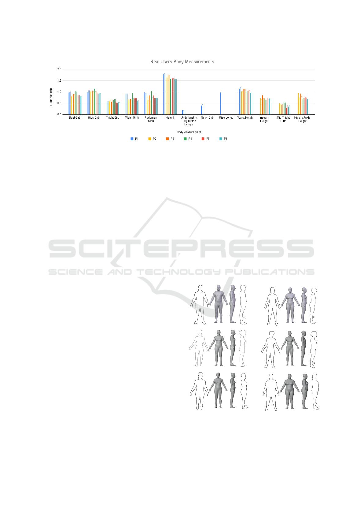
Figure 3: Real users’ final measurements. Each subject corresponds to a different color. The solid bar denotes the actual
measurement value (ground truth of a specific person) and the hollow one its estimated value. To simplify the comparison, we
show each user’s original measurement value and the estimated one. We evaluated the top ten measurements of each gender,
represented in Table 1. There are six common measurements, while the last four are gender-specific.
Body Shape. To evaluate the body shape, we took
two pictures of the users: a frontal and a profile one
and extracted their silhouette. Finally, these images
were placed side by side with their estimated. In
Figure 4 we can see the final results. We noticed
that our model had difficulty modeling the waist of
estimated shapes. In cases where the original shape
had hips relatively larger than the waist, as P3 does,
our model returned a shape with a larger waist than
it should. However, our model estimated shapes
with a waist relatively similar to the hips as having
smaller waists. The data set contains the most typical
shape variations: A more slim appearance for both
represented genders and a waist thinner than the hip
for females. This made possible for our model to
return better estimations regarding P1, P2, P3, P4
and P5. Since P6 belongs to a group that is poorly
represented in the dataset, the model struggled to
estimate its shape. Our model also had difficulties
estimating fuller thighs. P2 is a good example.
We see that the frontal silhouette had fuller thighs,
something that the estimation does not. However, the
interior of the thighs is not very similar. However,
the estimations returned new shapes that were pretty
similar to the original ones. We asked subjects
whether the estimation was similar to their bodies.
They pointed the issues that we related in this paper
but said that overall the estimated shapes looked like
them. We concluded that our model could correctly
estimate body shapes from a few body measurements.
Body Measurements. We evaluated the body mea-
surements of the estimations and compared them with
the original ones and the results obtained from mea-
suring estimations are represented in Figure 3. We
noticed that the estimated height and waist height
measurements in female estimations were the same
as the original ones. However, the other height mea-
surements had some errors associated because people
found it difficult to understand how to measure them-
selves. Other slight errors may be associated with the
fluctuation of the waist point in the dataset meshes.
The measurement that had more error associated was
abdomen girth, with a distance difference reaching
up to 31cm. We believe this is also because the ver-
tex fluctuations on the meshes and the girth extracted
might sometimes be more similar to the waist than the
abdomen itself. The estimations of the bust girth were
usually smaller than the original, reaching a distance
difference of 5cm in the worst case. However, some
measurements did not behave like this: thigh girth and
mid-thigh girth estimations had a higher measurement
value than the original value.
Figure 4: Visual comparison of real users silhouette with
their correspondent shape estimation using the top 8 mea-
surements subset. From left to right and top to bottom we
called these estimations P1, P2, P3, P4, P5 and P6.
GRAPP 2022 - 17th International Conference on Computer Graphics Theory and Applications
324

5 CONCLUSIONS
We compared two models, one using PCA weights
and the other using linear transformations to esti-
mate new shapes and concluded that PCA weights
are less adequate to estimate body shapes from mea-
surements. While evaluating with real users, we es-
timated our linear model using our top eight subsets.
Then, similarly to the validation step, we evaluated
the resulting body shape and measurement estima-
tions. We conclude that our model is not appropri-
ate for estimating new shapes with similar body mea-
surements as the original form. Moreover, since we
aim to develop a virtual dressing room, there are con-
cerns about how similar the estimated shape is to the
actual user body. If the measurements differ, instead
of helping people, our technique may mislead them
into buying the wrong size clothes. On the other side,
our model provided new body shapes that were very
similar to the original ones. The users also supported
this because the majority said that the estimation had
a similar shape to theirs. Our models can then sim-
ulate garment fitting and rendering in virtual dress-
ing rooms. Future work includes estimating measure-
ments from a single photograph for a more expedited
user experience.
ACKNOWLEDGEMENTS
The work reported in this article was partly supported
by national funds through Fundac¸
˜
ao para a Ci
ˆ
encia e
a Tecnologia (FCT) under project UIDB/50021/2020.
REFERENCES
Anguelov, D., Srinivasan, P., Koller, D., Thrun, S., Rodgers,
J., and Davis, J. (2005). Scape: Shape completion
and animation of people. In ACM SIGGRAPH 2005
Papers, SIGGRAPH ’05, page 408–416, New York,
NY, USA. Association for Computing Machinery.
Aubel, A. and Thalmann, D. (2000). Realistic deformation
of human body shapes. In Magnenat-Thalmann, N.,
Thalmann, D., and Arnaldi, B., editors, Computer An-
imation and Simulation 2000, pages 125–135, Vienna.
Springer Vienna.
Baek, S.-Y. and Lee, K. (2012). Parametric human body
shape modeling framework for human-centered prod-
uct design. Computer-Aided Design, 44(1):56 – 67.
Digital Human Modeling in Product Design.
Chen, Y., Song, Z., Xu, W., Martin, R. R., and Cheng, Z.-
Q. (2019). Parametric 3d modeling of a symmetric
human body. Computers & Graphics, 81:52 – 60.
Dibra, E., Jain, H.,
¨
Oztireli, C., Ziegler, R., and Gross,
M. (2016). Hs-nets: Estimating human body shape
from silhouettes with convolutional neural networks.
In 2016 Fourth International Conference on 3D Vision
(3DV), pages 108–117.
Dijkstra, E. W. (1959). A note on two problems in connex-
ion with graphs. Numerische mathematik, 1(1):269–
271.
Goldman, S. (2021). Post-pandemic e-commerce: The un-
stoppable growth of online shopping.
Iwamoto, N., Shum, H. P. H., Yang, L., and Morishima,
S. (2015). Multi-layer lattice model for real-time dy-
namic character deformation. Computer Graphics Fo-
rum, 34(7):99–109.
Kanazawa, A., Black, M. J., Jacobs, D. W., and Malik,
J. (2018). End-to-end recovery of human shape and
pose. In Proceedings of the IEEE Conference on Com-
puter Vision and Pattern Recognition (CVPR).
Loper, M., Mahmood, N., Romero, J., Pons-Moll, G., and
Black, M. J. (2015). Smpl: A skinned multi-person
linear model. ACM Trans. Graph., 34(6).
Pezzini, G. (2021). Why physical stores are still vital for
retail.
Pratscher, M., Coleman, P., Laszlo, J., and Singh, K.
(2005). ¡i¿outside-in¡/i¿ anatomy based character
rigging. In Proceedings of the 2005 ACM SIG-
GRAPH/Eurographics Symposium on Computer An-
imation, SCA ’05, page 329–338, New York, NY,
USA. Association for Computing Machinery.
Saito, S., Simon, T., Saragih, J., and Joo, H. (2020). Pi-
fuhd: Multi-level pixel-aligned implicit function for
high-resolution 3d human digitization. In Proceed-
ings of the IEEE Conference on Computer Vision and
Pattern Recognition.
Seo, H. and Magnenat-Thalmann, N. (2003). An automatic
modeling of human bodies from sizing parameters. In
Proceedings of the 2003 Symposium on Interactive 3D
Graphics, I3D ’03, page 19–26, New York, NY, USA.
Association for Computing Machinery.
Volz, A., Blum, R., H
¨
aberling, S., and Khakzar, K. (2007).
Automatic, body measurements based generation of
individual avatars using highly adjustable linear trans-
formation. In Duffy, V. G., editor, Digital Hu-
man Modeling, pages 453–459, Berlin, Heidelberg.
Springer Berlin Heidelberg.
Wuhrer, S. and Shu, C. (2012). Estimating 3d human shapes
from measurements. Machine Vision and Applica-
tions, 24(6):1133–1147.
Yang, Y., Yu, Y., Zhou, Y., Du, S., Davis, J., and Yang,
R. (2014). Semantic parametric reshaping of human
body models. In 2014 2nd International Conference
on 3D Vision, volume 2, pages 41–48.
Zhang, T., Wang, J., Zhu, Q., and Yin, B. (2020). See
through occlusions: Detailed human shape estimation
from a single image with occlusions. In 2020 IEEE In-
ternational Conference on Image Processing (ICIP),
pages 2646–2650.
Zhu, H., Zuo, X., Wang, S., Cao, X., and Yang, R. (2019).
Detailed human shape estimation from a single image
by hierarchical mesh deformation. In Proceedings of
the IEEE/CVF Conference on Computer Vision and
Pattern Recognition (CVPR).
Estimating Body Shapes from Measurements
325
