
A Formally Correct and Algorithmically Efficient
LULC Change Model-building Environment
Franc¸ois-R
´
emi Mazy
1 a
and Pierre-Yves Longaretti
1,2 b
1
Universit
´
e Grenoble Alpes, CNRS, Inria, Grenoble INP, LJK, 38000 Grenoble, France
2
Universit
´
e Grenoble Alpes, CNRS-INSU, IPAG, CS 40700, 38052 Grenoble, France
Keywords:
Land Use Change, Land Cover Change, LULC, Model Development, Model Evaluation, Model Accuracy,
Density Estimation, Calibration, Allocation, Map Simulation.
Abstract:
The use of spatially explicit land use and land cover (LULC) change models is widespread in environmental
sciences and of interest in public decision-help. However, it appears that these models suffer from significant
biases and shortcomings, the sources of which can be mathematical, conceptual or algorithmic. We formalize
a modeling environment that distinguishes a calibration-estimation module and an allocation module. We
propose an accurate calibration-estimation method based on kernel density estimation and detail an unbiased
allocation algorithm. Moreover, a method of evaluation of LULC change models is presented and allows us
to compare them on various fronts (accuracy, biases, computational efficiency). A case study based on a real
land use map but with known (enforced) transition probabilities is used. It appears that the estimation error of
the methods we propose is substantially improved over the best existing software. Moreover, these methods
require the specification of very few parameters by the user, and are numerically efficient. This article presents
an overview of our LULC change modeling framework; its various formal and algorithmic constituents will
be detailed in forthcoming papers.
1 INTRODUCTION
Land use and land cover (LULC) change is a ma-
jor driver of global change alongside the more vis-
ible issues of climate change and biodiversity loss.
The study of LULC change is of major interest
in analyzing and understanding a variety of socio-
environmental phenomena but also for decision-help
on mitigation and adaptation policies, and the litera-
ture on LULC change studies is by now quite substan-
tial. Different LULC change modeling strategies have
been developed over the last few decades to address
these research issues (static, dynamic, agent-based,
local or global scale, etc. . . ).
In the present work, we focus on spatially explicit,
statistical LULC change model building. Such mod-
els generally consists of estimating transition proba-
bilities from one land-use state to another based on
(usally) two land-use maps at different dates that re-
flect changes in the past. These models are designed
to simulate new land use maps, in scenario-driven
projections of future land use and cover. Such allo-
a
https://orcid.org/0000-0001-8405-0141
b
https://orcid.org/0000-0002-4940-0756
cated maps can be used for a variety of purposes. For
example, they may be coupled to models of ecosys-
tem services to produce evaluations of their future
evolution. In fact, producing accurate spatially ex-
plicit projections of the effects of public decisions
bearing on social-ecological problems is a current is-
sue for such models (Verburg et al., 2019).
Statistical and spatially explicit LULC change
models constitute a popular approach to LULC
change modeling, and various model-building soft-
ware have already been devised in this framework.
Among the most well-known, one may quote Di-
namica EGO (Soares-Filho et al., 2002), Idrisi LCM
(Eastman et al., 1995), or the CLUE family of mod-
els (Verburg et al., 1999), the last member being
CLUMondo (van Vliet et al., 2015). However, these
software (and others) exhibit substantial differences
in results for the same case studies (Mas et al.,
2014; Prestele et al., 2016; Alexander et al., 2017),
which raises an important concern on the reliability
of the LULC change modeling process itself.
No study to date has clearly identified the origin of
the differences of behavior and outcome displayed by
the existing model-building software on a same prob-
Mazy, F. and Longaretti, P.
A Formally Correct and Algorithmically Efficient LULC Change Model-building Environment.
DOI: 10.5220/0011000000003185
In Proceedings of the 8th International Conference on Geographical Information Systems Theory, Applications and Management (GISTAM 2022), pages 25-36
ISBN: 978-989-758-571-5; ISSN: 2184-500X
Copyright
c
2022 by SCITEPRESS – Science and Technology Publications, Lda. All rights reserved
25
Calibration
Land use at t
0
Land use at t
f
Explanatory variables at t
0
Estimation
Scenario for a time step dt
Explanatory variables at t
s
Land use at t
s
Allo cation
Allocated land use
at t
s
+ dt
iteration
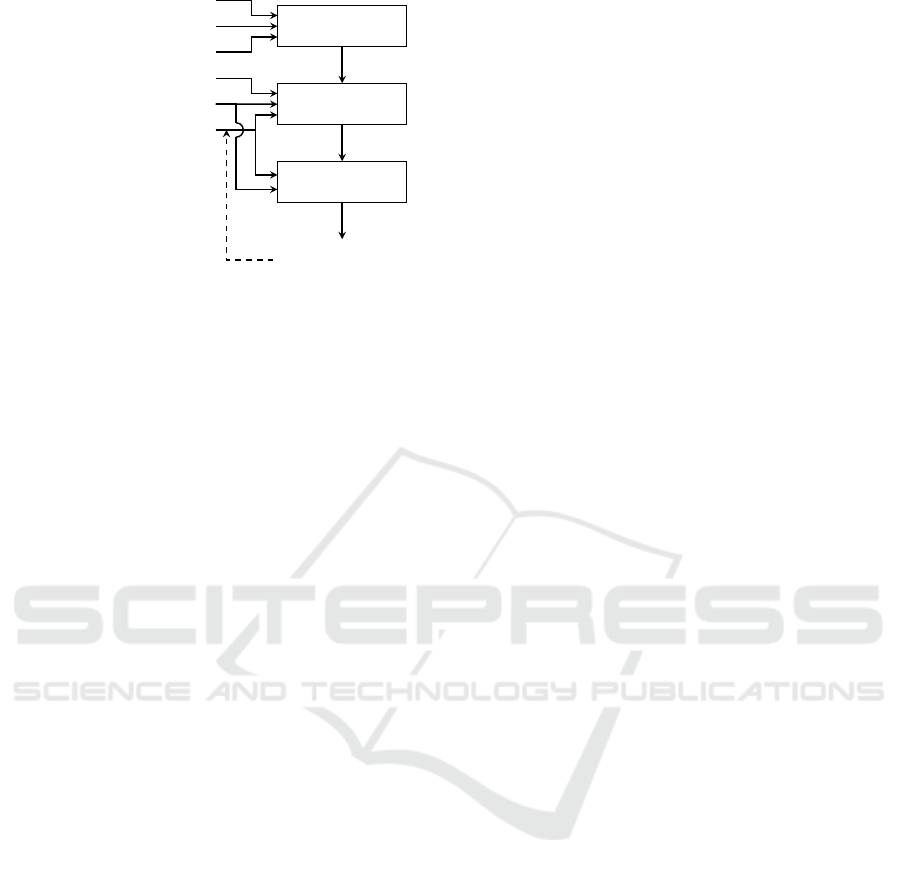
Figure 1: General architecture of a spatially explicit statis-
tical LULC change model.
lem, let alone proposed a formally correct theoretical
framework for this type of LULC change modeling.
Moreover, comparing different LULC change models
on their spatial outcomes is a poorly mastered opera-
tion in the literature (van Vliet et al., 2016) and more
precise evaluation methods are needed. Nevertheless,
as will be illustrated in the course of this work for
the three modeling environment just mentioned, these
discrepancies can be traced to differences in the for-
mal and algorithmic choices made in their elabora-
tion. In fact, quite a few of these choices were made
without paying sufficient attention to the constraints
imposed by a correct ab initio formal investigation of
the probabilistic foundation of the problem, leading
to a number of errors and biases.
More precisely, we address these issue by focus-
ing successively on the calibration-estimation and al-
location processes in order to propose a fully formal-
ized and conceptually correct foundation for statisti-
cal spatially explicit LULC change analyses. We also
provide efficient and bias-free algorithmic implemen-
tations of these processes, which constitute the core of
this approach to LULC change model-building. The
present work illustrates some of our main results on
these two fronts. A detailed exposition of the un-
derlying formal analyses and algorithmic implemen-
tations will be given in forthcoming dedicated papers.
The first one will formalize in a rigorous ways statis-
tical LULC changes by groups of contiguous pixels
(patches), starting from the more common pixel by
pixel probability distributions, and introduce an allo-
cation algorithm to this effect, that will be explicitly
shown to be bias-free. The second one will be ded-
icated to the calibration and estimation of probabil-
ity transitions. Finally, the last article will provide a
systematic method of identification and a systematic
analysis of the biases present in the software men-
tioned above.
This paper is organized as follows. The typical
structure of statistical spatially explicit LULC change
models is recalled in section 2. Next, a new and
accurate calibration-estimation method and an unbi-
ased allocation methods are briefly overviewed in sec-
tion 3. We then propose an evaluation method for
LULC change models that allows us to compare their
results and performances; the most salient features are
described in section 4. The next section introduces
a case study to illustrate the methods of the previ-
ous sections, and presents some of our results (sec-
tion 5). Finally, the last section summarizes these
findings along with other important results on these
issues that will be established in our forthcoming pa-
pers on the topic.
We assume that a number of preliminary model-
ing choices are made prior to the comparison of per-
formances mentioned right above: elaboration of the
LUC typology, choice of explanatory variables, and
choice of the discretization (pixel) scale. Thus, we
exclude from the perimeter of our analysis the obvi-
ous influence of these choices on the results (Garc
´
ıa-
´
Alvarez et al., 2019).
2 LULC CHANGE MODEL
ARCHITECTURE
Spatially explicit statistical LULC change models
are generally (but not always) organized around two
main modules: calibration-estimation, and allocation
(Fig. 1). This allows us to investigate in turn their
underlying logic, formal foundation and algorithmic
implementation.
2.1 Calibration-estimation Module
We start from two raster (i.e., pixelized) LULC maps
at two different dates t
0
and t
1
as well as maps of
the d explanatory variables of interest, characterizing
LULC changes (e.g., altitude, distance to the roads,
etc. . . ). Pixel sizes can vary from a few meters to a
few tens of kilometers depending on case studies; the
largest maps may involve tens of millions of pixels.
The dates t
0
and t
1
differ typically by a few years.
Although changes occur in patches of contiguous
pixels, the calibration-estimation process focuses on
individual pixel probability distributions; patches are
then produced on this basis in the allocation module.
Pixels undergo a change from land use u to land use v.
Each pixel i is characterized by a collection (vector or
tuple) z
i
of values of the d explanatory variables. The
transition probability distribution must be evaluated
for all possible explanatory variables combinations y
present in the calibration maps, including those which
GISTAM 2022 - 8th International Conference on Geographical Information Systems Theory, Applications and Management
26

were not observed to undergo a transition but may be
expected to in the future. To this effect, one needs
to evaluate the conditional pixel transition probabil-
ity P(v|u, y). This involves a form of interpolation in
explanatory variable space, called estimation (Fig. 1).
2.2 Allocation Module
A new land use map is simulated from an initial one
(possibly different from the calibration maps), from
the explanatory variables (when needed) and from the
probability of land use change maps for each possible
LULC state change (Fig. 1). Allocations are made in
groups of contiguous pixels (patches). The process in-
volves a sampling algorithm and attributes a possible
new LULC state on the basis of the associated tran-
sition probability distribution and some patches con-
straints. The map obtained in this way is a particu-
lar instantiation of this probability distribution; many
others could have been produced for the same time
step, and all such maps are statistically equivalent, ex-
cept for statistical noise. This point is usually ignored
in existing model-building environments, although it
is crucial to identify errors and biases, as will be dis-
cussed later on. The details of our patch construction
method are involved but not critical for software per-
formance comparison (both in terms of accuracy and
execution time) and will therefore not be presented
here.
In the process the user provides a transition ma-
trix that characterizes the rates of change per time step
between each land use state, and characterized by an
overall probability P(v|u) for all possible LULC ini-
tial and final states u,v. This matrix is usually speci-
fied through scenarios.
2.3 Existing LULC Change
Model-building Environments
In the present work we focus on three of the most
widely used software (van Vliet et al., 2016): Dinam-
ica EGO, Idrisi LCM and CLUMondo. Our objective
is to contrast their performances (accuracy and com-
putational efficiency) to the modeling strategy and al-
gorithmic implementation we propose in the next sec-
tion.
Dinamica EGO fits reasonably well in the archety-
pal structure of Fig. 1. Transition probabilities are
usually estimated from the use of weights of evi-
dence, applied after binning the user-defined explana-
tory variables (Soares-Filho et al., 2002). This bin-
ning step requires to specify a number of parame-
ters, which turn out to have a very strong impact
on the obtained results. Moreover, this method of
estimat- ing transition probabilities is based on the
strong assumption of statistical independence of the
explanatory variables; it turns out that even modest
amounts of cross-correlation between these variables
may lead to non negligible errors in the estimated
transition probabilities. This software implements
an allocation method relying on a pixel pre-selection
process (pruning), implemented to reduce computa-
tional time); such pruning also produces significant
biases in the results.
Idrisi LCM (Eastman et al., 1995) also im-
plements a calibration/allocation architecture, while
leaving the user with less control on modeling choices
than Dinamica EGO. This strategy is adopted on pur-
pose, in order for users with little expertise to never-
theless be able to implement a LULC change model.
The particular LCM version we have used is the one
bundled in Idrisi Selva. This software proposes differ-
ent models for estimating transition probabilities: lo-
gistic regression (LCM LR), SimWeight (LCM SW)
and Multi-Layer Perceptron (LCM MLP). The LCM
allocation module is very simple and deterministic, as
the allocation algorithm implemented in this software
essentially ignores the statistical nature of the process.
This results in simple but strongly biased allocation
rules.
Finally, the CLUE family of software (Verburg
et al., 1999), the latest of which is CLUMondo (van
Vliet et al., 2015), chooses to estimate the probabili-
ties of change from a single land use map, from which
it defines transition probabilities through a logistic re-
gression on all explanatory variables. Also, CLU-
Mondo does not allow the modeler to access its al-
location module independently.
3 CLUMPY: A NEW LULC
CHANGE MODEL-BUILDING
ENVIRONMENT
We present here in a succinct manner the meth-
ods used in our calibration-estimation and alloca-
tion modules. The closest analog in the existing
model-building environments is Dinamica EGO. The
main differences come from our more sophisticated
but more accurate and efficient calibration-estimation
method, our demonstrably error- and bias-free allo-
cation method, and significantly more efficient al-
gorithms leading to substantial gains in computation
time in large problems.
These modules constitute the core of our model-
building environment, called CLUMPY (Comprehen-
sive Land Use Model in Python).
A Formally Correct and Algorithmically Efficient LULC Change Model-building Environment
27

3.1 Calibration-estimation
3.1.1 Bayes Rule
The probability of transition from land use u to land
use v of a pixel characterized by the d-tuple of ex-
planatory variables y is noted P(v|u,y). This nota-
tion emphasizes the fact that this probability is con-
ditioned by the knowledge of the values of u and y.
Bayes rule allows us to express this probability in a
more convenient way for calibration purposes:
P(v|u,y) = P(v|u)
p(y|u,v)
p(y|u)
. (1)
The various factors on the right-hand side member
are defined as follows. P(v|u) is the global transi-
tion probability, specified by a scenario provided by
the user. This quantity can also be computed directly
from the observed transitions between the calibration
maps at times t
0
and t
1
. Next, p(y|u) is a condi-
tional probability density. We use probability densi-
ties because explanatory variables are usually contin-
uous quantities, and we do not bin them in the end,
in order to produce a more accurate calibration pro-
cedure. By definition p(y|u)dy is the probability of
observing y within the small volume dy of explana-
tory variable space, for pixels of initial state u. Simi-
larly, p(y|u,v) is the probability density of y for pix-
els making the transition from states u to v. Note that
the calibration process, which is based on observed
transitions, uses these probabilities in the frequency
of occurrence meaning, while the allocation module
applies Bayes rule in a Bayesian sense.
The interest of using Bayes rule lies in the fact that
p(y|u) and p(y|u,v) are much simpler to estimate than
P(v|u,y). Indeed, it is then a question of estimating
density functions on y for a set of pixels of initial state
u for p(y|u) or potentially undergoing a LULC state
transition from u to v for p(y|u,v). This problem is
widely addressed in machine learning and is called
density estimation.
Consider a set of n calibration pixels, made of
all the pixels that actually underwent a LULC state
change from u to v and are directly extracted from two
calibration maps at time t
0
and t
1
. Each of these pixels
is characterized by its explanatory variables noted z.
We wish to estimate the transition probability of all m
pixels in our maps; these are by definition evaluation
pixels. Each of these pixels is characterized by its ex-
planatory variables noted this time y. The problem is
therefore to estimate P(v|u,y).
The idea is to calibrate a density estimator with the
calibration pixels for both probability densities and
then to estimate these probability densities for all pix-
els with the obtained density estimator. Finally, as the
global transition probability P(v|u) is given, we can
apply Bayes rule to obtain P(v|u,y).
3.1.2 Density Estimation by Kernel Density
Estimator (KDE)
Estimating a probability density is a widely addressed
problem in the machine learning literature (Scott,
2015). A simple and not very precise method is to
make histograms in explanatory variable space. This
requires to bin explanatory variables; unfortunately,
the choice of the bin size has a strong impact on
the results. Some related methods such as averaged
shifted histograms have been proposed to circumvent
the problem (Chamayou, 1980).
More sophisticated methods perform density es-
timates by positioning a kernel function K charac-
terized by a user-specified width parameter h (called
bandwidth) on each calibration data point and sum-
ming over all these kernels at the desired locations
of estimation (in explanatory variable space). This
is called kernel density estimation (Wand, 1992), or
KDE in short. This very efficient method is how-
ever highly computationally intensive as soon as the
number of explanatory variables and elements (here,
pixels) increases. Many kernel functions may be
studied (e.g., gaussian kernels), and various methods
have been proposed to approximate the resulting fam-
ily of estimators (O’Brien et al., 2016; Charikar and
Siminelakis, 2017). However, these relatively com-
plex methods often require large amounts of mem-
ory since they allocate full matrices representing the
entire space of explanatory variables. Thus, when
confronted with more than a few explanatory vari-
ables, these methods can be inapplicable due to lack
of memory space on standard machines; the compu-
tation time also increases quite fast with the number
of dimensions.
Instead, we implemented a hybrid binning/KDE
method, that keeps part of the simplicity of simple
histograms with only a small degradation of the per-
formance of pure Kernel density estimator methods.
The binning is performed on a scale h/q smaller than
the bandwidth h (Wells and Ting, 2019), where q > 1
is an odd integer. A kernel density estimator is then
applied to the small bins themselves instead of the
original individual elements (pixels) in explanatory
variable space. One can then show that the larger
q, the smaller the approximation error. This hybrid
method maintains the spirit of continuous density es-
timation, while being much more computationally ef-
ficient than direct KDE estimators (both in terms of
computational time and memory use). This is what
we used in our estimations of P(y|u) and P(y|u, v).
The choice of the kernel width h for the KDE
GISTAM 2022 - 8th International Conference on Geographical Information Systems Theory, Applications and Management
28

method is a very important issue due to its influence
on the quality of the estimation. Indeed, choosing a
too narrow bandwidth results in an over-interpretation
of the observational data and in noisy estimates. On
the other hand, a too broad bandwidth leads to under-
fitting (or over-smoothing) and to a degradation of the
estimate of the probability density. The determina-
tion of the optimal width of the kernel is a non-trivial
problem and is widely discussed in the machine-
learning literature (Wand and Jones, 1994; Rudemo,
1982; Sain et al., 1994). However, these methods are
computationally very expensive as soon as the num-
ber of pixels is large and the number of dimensions
exceeds 3, which is very frequently the case in LULC
change studies.
This being said, in the LULC change context,
a slight over-smoothing is not a problem and can
even be interesting, because transition probabilities
are usually undersampled, and therefore noisy. Con-
sequently, we chose to determine the KDE bandwidth
h from the principle of maximum smoothing of Terrel
(Terrell, 1990), leading to
h
Terrel
=
(d + 8)
d+6
2
π
d
2
Z
K
2
16 n (d + 2) Γ
d+8
2
, (2)
where K is the kernel density estimator. The slight
oversmoothing involved turns out to be essentially un-
noticeable in our tests, while this prescription con-
siderably reduces the computational burden of KDE
methods.
We have checked on various test problems, and will
soon show, that even simple kernel functions (such
as a square box, a triangle or a gaussian kernel) give
much more accurate results than existing calibration
methods.
Note finally that, because explanatory variables
are of widely different nature and not statistically in-
dependent, it is necessary to normalize them in or-
der to work with data of zero mean and covariance
matrix equal to the identity in explanatory variable
space. This operation is called “whitening transfor-
mation” in the machine learning literature. It makes
it legitimate to use a unique bandwidth in all dimen-
sions in the transformed explanatory variable space
and greatly simplifies the numerical implementation
of our calibration-estimation method.
3.2 Allocation
In general, the allocation module takes as input a land
use map as well as the transition probability maps ob-
tained in the calibration-estimation module. The allo-
cation method presented here also requires the knowl-
edge of the explanatory variables of the input map.
The simulation of an allocated map produces a
specific statistical sampling of the transition proba-
bilities. So far, we have focused on pixel transition
properties. However, as already mentioned, we al-
locate pixel patches. Following the logic initiated in
Dinamica EGO, a first pixel is selected according to
the transition probability distribution obtained by our
calibration-estimation procedure. This pixel is called
a “core pixel” or “pivot-cell”. Then, a specific pro-
cedure is applied to create a patch around this core
pixel. This procedure is characterized by different pa-
rameters such as the surface of the patch, and its elon-
gation. Patches created in this way reproduce some
of the statistical properties of actually observed tran-
sition patches, but are defined algorithmically to pro-
vide some randomness in their shape.
The allocation modules implemented in the ex-
isting software turn out to be all biased to various
extents. Such biases have not yet been identified in
the literature, first because a biasing criterion has not
been formulated, and second because the details of
these software allocation procedure is not fully docu-
mented. We have circumvented this last problem by a
combination of literature analysis, educated guesses,
retro-engineering, questions to model developers, and
re-implementation (when feasible) of these allocation
algorithms to check that our understanding of their
structure and content exactly reproduces the outcome
of the original software on a number of test problems.
We have also formulated a simple but powerful “no-
bias” criterion, which, in essence, requires that the
post-allocation probability distributions are identical
to the pre-allocation ones. This is in fact more of an
unavoidable self-consistency requirement, but it turns
out that none of the existing LULC change model-
building software does satisfy it.
This allowed us to implement a strategy of sys-
tematic identification and characterization of the var-
ious biases present in existing model-building soft-
ware. We illustrate this process on a particularly im-
portant bias related to pruning, relying on an efficient
bias-free algorithm which avoids the need for prun-
ing.
3.2.1 Pruning
LULC change models may involve a very large num-
ber of pixels (e.g., tens of millions). Therefore, it can
be interesting to pre-select a limited number of pixels
in order to speed up the allocation procedure. This
pre-selection is called pruning and is implemented by
Dinamica EGO and LCM in two different ways, both
of which turn out to be significant sources of bias.
Dinamica EGO’s pruning method consists in rank-
ing pixels by decreasing order of transition probabil-
A Formally Correct and Algorithmically Efficient LULC Change Model-building Environment
29

ity P(v|u,y). Pixels are then pre-selected in this or-
der in this list; the number of pre-selected pixels is
equal to the number of pixels necessary to reach the
targeted LULC change surface defined by the user se-
lected scenario, multiplied by a pruning parameter F.
The default value is F = 10 (ten times as many pixels
as needed for the various transitions are pre-selected).
LCM ranks the pixels by decreasing order of
the probability density (or probability distribution if
binned) of the explanatory variables for this transi-
tion, p(y|u, v). Then LCM keeps the exact number
of pixels that are necessary to reach the targeted tran-
sition surface defined by the selected scenario, and
has a specific procedure to resolve conflicts of al-
location for the same pixel. Thus, LCM’s pruning
method is also its allocation method since all pixels
selected in this way are directly allocated without any
further consideration. This procedure has the advan-
tage of simplicity and ensures that transitions occur
in patches (due to the spatial continuity of the ex-
planatory variables probability densities). However,
the maps allocated by LCM often suffer from a se-
vere lack of realism, and they always violate our self-
consistency no-bias requirement.
Although establishing which probability ordering
should in principle be used for pruning is not an
obvious task, we have proved that LCM’s choice
[p(y|u,v)] is the theoretically correct one; this ap-
plies although the correct allocation probability dis-
tribution is by definition P(v|u, y). This being said,
both Dinamica EGO and LCM pruning strategies are
strongly biased because they modify to various ex-
tents the probability distributions which should be en-
forced exactly. LCM is the more biased of the two, al-
though Dinamica EGO has chosen an incorrect prob-
ability ordering for pruning.
An unbiased pruning method necessarily con-
sists in a random sampling performed according to
p(y|u,v), and selects the number of kernel pixels
needed to reach the targeted number of transited
pixels. Thus, the probability distribution of this
pixel subsample will be statistically representative of
p(y|u,v) and there will be no unwarranted truncation
of this probability density distribution.
The motivation for applying a pruning procedure
lies in the numerical acceleration of the allocation
method for a very large number of pixels. How-
ever, the implementation in Python of the our allo-
cation procedure as presented in section 3.2.2 proves
to be numerically very efficient without pruning, even
though the number of pixels in some of our case stud-
ies is very large (> 10
8
); this efficiency relies on
the use of dedicated Python functions, which perform
nearly as fast as equivalent C codes. Still, we have de-
signed a bias-free pruning algorithm, for possible use
in particular problems.
3.2.2 Unbiased Allocation
In addition to pruning, other biases can occur in the
allocation procedure. In particular, the creation of
patches around a core pixel automatically excludes
these patch pixels from the rest of the allocation pro-
cedure. However, they could just as well be selected
afterwards.
In order to resolve such potential conflicts, we de-
signed the following iterative allocation procedure for
a given initial land use state :
1. We know the transition probability P(v|u,y) of
each pixel for all (u,v). We can therefore apply
a generalized Von Neumann rejection sampling,
which allows us to test all possible states v at the
same time for any given u. We obtain an unbiased
sample of kernel pixels for each of the transitions
studied. If no kernel pixel is selected, the alloca-
tion procedure is terminated at this point.
2. A single kernel pixel is randomly and uniformly
drawn; its associated transition has been deter-
mined in the previous step.
3. The procedure of patch creation around this core
pixel is applied next. The selected pixels are actu-
ally allocated on the simulated map.
4. P(v|u) is updated, taking into account that a cer-
tain number of pixels have already been allocated.
This probability is therefore reduced for the rest
of the allocation procedure in the considered time
step.
5. p(y|u) is updated next because some elements
have already been allocated, which has modified
the probability density distribution of the explana-
tory variables.
6. p(v|u,y) is then recalculated from Bayes rule
Eq. (1); the probabilities involved in steps 4 and
5 are also updated. We then start again at step 1.
We have shown that a carefully designed algorithm
of this type is bias-free. This procedure is however
demanding since it requires to re-estimate very fre-
quently p(y|u). We therefore update this probabil-
ity distribution only when the percentage of allocated
pixels is significant enough that the estimated prob-
ability is too far from the real distribution (in prac-
tice, after a fixed small percentage of state changes
has been achieved). This may introduce a slight bias.
GISTAM 2022 - 8th International Conference on Geographical Information Systems Theory, Applications and Management
30

4 EVALUATION
A review of the literature shows that validating the re-
sults obtained by LULC change models is an uncom-
mon practice. This deficiency underlies some of the
doubts that may be raised on the robustness of LULC
change modeling (van Vliet et al., 2016). In any case,
before specific results may be validated, the modeling
framework itself should be validated. A first attempt
along these lines has already been carried out on artifi-
cal data (Mas et al., 2014) but the lack of exact knowl-
edge of the transition probabilities involved precluded
any detailed evaluation of the LULC change models
that were tested in this earlier work. Indeed, one of
the main problems of statistical LULC change mod-
eling is the estimation of the probability distribution
P(v|u,y) (section 3.1), and, furthermore, it is impos-
sible to know this probability distribution exactly in a
real case study. Validating this estimation of P(v|u,y)
therefore remains an essential objective.
We propose here a simultaneous validation
method for the calibration-estimation and global
calibration-estimation/allocation procedures, that al-
lows us to objectively compare different model-
building strategies. This is achieved by quantifying
the difference between the transition probabilities ob-
tained from our hybrid KDE estimation in the cali-
bration phase or in the post-allocation one, and ex-
actly specified pre-calibration transition probabilities.
We may proceed to this effect from semi-real or com-
pletely artificial data. We start from a (real or artifi-
cial) LULC map at t = t
0
. We adopt an exactly known
transition probability distribution, P
∗
(v|u,y). This ex-
act transition probability may be defined analytically
or numerically. Then, a new LULC map at time t = t
1
is produced with our allocation procedure (based on
this exact probability distribution and our patch cre-
ation algorithm).
This allows us to implement two validation pro-
cesses:
Calibration-estimation Comparison. We select a
calibration-estimation method from an existing
LULC change model-building environment, and
produce from the two maps just specified at t
0
and t
1
an estimate
ˆ
P(v|u,y) of P
∗
(v|u,y). We re-
peat this process for all the calibration methods
we want to compare, including ours.
Calibration-estimation/Allocation Comparison.
We now wish to evaluate the relative efficiencies
of these modeling environments over the whole
calibration-estimation/allocation process. We
thus use as inputs the LULC map at t = t
1
and the
probability distribution
ˆ
P(v|u,y) determined by
the previously described calibration-estimation
comparison process, for any of the model-
ing environments tested. We produce next a
new LULC map at t = t
2
from the associated
allocation procedure. We recover a new post-
allocation estimate
˜
P(v|u,y) of P
∗
(v|u,y) from
the calibration-estimation method of the same
modeling environment. We repeat this process
for all the modeling environments we want to
compare, including ours.
The comparison of the exact (enforced) probability
distribution with the estimated ones can be done in
various and more or less sophisticated ways. In this
article, we limit ourselves to two very simple ap-
proaches. The first one consists in producing graphs
of the estimated distributions
ˆ
P(v|u,y) and the ex-
act one P
∗
(v|u,y) considered as a function of y, for
various one-dimensional cuts in explanatory variable
space, e.g., by fixing all explanatory variables but one.
This gives a direct check of the accuracy of the var-
ious methods, but only on a limited (although ran-
domly chosen) set of locations in explanatory variable
space.
The second validation method is more global and
consists in calculating the average of the absolute er-
ror throughout explanatory variable space:
ε
calib
=
1
m
m
∑
i=1
P
∗
(v|u,y
i
) −
ˆ
P(v|u,y
i
)
,
ε
tot
=
1
m
m
∑
i=1
P
∗
(v|u,y
i
) −
˜
P(v|u,y
i
)
(3)
where m is the number of pixels where the dif-
ference is evaluated (generally, all pixels concerned
by the u → v transition in a map), and where
the subscript “calib” or “tot” refers either to the
calibration-estimation comparison process or to the
global calibration-estimation/allocation one.
By construction Eq. (3) tends to underesti-
mate large but localized differences. Using one-
dimensional cuts minimizes this possibility to some
extent. We could also, e.g., identify the largest abso-
lute difference, and count the number of pixels where
this difference is achieved within a given tolerance.
We avoid relative differences because they might be
very large where the transition probability is low, but
this would not necessarily reflect a notable inaccuracy
in the estimation itself.
In any case, we can measure the difference be-
tween the exact and estimated probability distribu-
tions, a validation test that has been never been per-
formed so far, and thus have a first global evalua-
tion of the relative robustness of various calibration-
estimation and allocation modules (ours as well as
the ones implemented in existing model-building soft-
ware).
A Formally Correct and Algorithmically Efficient LULC Change Model-building Environment
31

Our own calibration-estimation and allocation
procedures are tested simultaneously and not inde-
pendently in both comparison processes (as the sec-
ond map needed in these tests is produced by our al-
location procedure). One may therefore ask whether
they are both validated in this way. Several lines of
arguments show that this is the case, relying on a pri-
ori and a posteriori analyses. First, we have formally
proved that our allocation procedure is bias-free (the
proof will be given elsewhere), i.e., that it enforces the
correct transition probability distribution. Also, the
KDE density estimation procedures have been shown
to converge exactly to the correct density distribu-
tion in the machine-learning literature in the limit of a
large number of available points (this form of conver-
gence is weaker than for allocation, but still relevant).
This applies also to our own hybrid KDE calibration-
estimation method, except possibly close to bound-
aries in explanatory variable space due to the kernel
truncation correction applied there (not described in
our overview of the method). Second, the numeri-
cal efficiency of our algorithms allow us to produce a
large number (thousands) of calibration-allocation se-
quences for the same time step in a reasonable compu-
tation time. We checked on a number of test problems
that post-allocation transition probabilities (recovered
by our calibration-estimation procedure) converge in
expectation value to the enforced one by averaging
over these multiple allocations. These arguments pro-
vide an a posteriori validation of both procedures. In-
deed, having errors or biases introduced by one pro-
cedure nearly exactly compensated by the other is be-
yond unlikely, considering the very different strate-
gies used in their elaboration.
A similar concern may be raised about the fact
that using our own allocation procedure to produce
the t = t
1
LUC map for testing calibration-estimation
procedures may favor our method over the others.
This concern is misplaced for the same type of rea-
son: the way this second map was produced is irrel-
evant precisely because there is no relation between
our allocation procedure and any of the calibration-
estimation procedures we have tested. Also, we have
just shown (or at least convincingly argued, until
the above-mentioned proofs are available in print),
that our allocation procedure produces unbiased post-
allocation probability distributions, so that the amount
of bias (due in fact to statistical noise) produced on a
single t = t
1
map is limited. In any case, it applies
equally to all tested calibration methods, which are
therefore treated on the same footing in this respect.
5 RESULTS AND DISCUSSION
In this section we apply the evaluation methods pre-
sented in section 4. We thus define a case study that
is intended to be representative of commonly encoun-
tered LULC change problems. We put to the test our
own modules (section 3) as well as the ones imple-
mented in the existing model-building software intro-
duced in section 2.3. The parameters used for each
model are specified in the Appendix.
5.1 Case Study Short Description
We are interested in a study area of 94 square kilo-
meters located in the Is
`
ere d
´
epartement in France.
We focus on a smaller sector in the Southwest of the
town of Grenoble; we have raster maps describing
this smaller area at 15 meters of resolution (6.3 mil-
lion pixels), and use 7 different land use classes at the
coarsest typology level (water bodies, mineral areas,
forests, agricultural areas, urban areas, economic ac-
tivity areas and other), and up to several tens at the
finest level. These data have been used in a recent
project, whose objective was to explore the future of
ecosystem services at the 2040 horizon under various
land planning scenarios (Vannier et al., 2016; Vannier
et al., 2019a; Vannier et al., 2019b).
For our present purposes, we only focus on a sin-
gle transition, namely from agricultural areas (u) to
urban areas (v). This is one of the main transitions re-
sponsible for urban sprawl. We chose this transition
for the sake of clarity and simplicity. The number of
agricultural area pixels is ∼ 3.3 million.
We have selected three explanatory variables to
characterize this transition: elevation above sea level
in meters (y
0
), slope in degrees (y
1
) and shortest dis-
tance from urban areas in meters (y
2
). These are three
of the main explanatory variables typically used in ur-
ban sprawl studies relying on statistical LULC mod-
elling frameworks.
In line with the evaluation strategy described in
section 4, we enforce a specific transition probability
distribution, namely we adopt a multivariate Gaussian
distribution:
P
∗
(v|u,y) =
N
µ,Σ
(y
0
,y
1
,y
2
) if {y
0
,y
1
,y
2
} ∈ D
0 else
(4)
where N
µ,Σ
refers to a normal distribution of mean
µ (vector of the means of the explanatory variables),
and covariance matrix Σ (covariance matrix of the ex-
planatory variables), (y
0
,y
1
,y
2
) is the vector of ex-
planatory variables, and D is a subset of the ex-
planatory variable space where the probability density
GISTAM 2022 - 8th International Conference on Geographical Information Systems Theory, Applications and Management
32

P(y|u) is larger than a (small) threshold (this avoids
potential problems in the application of Bayes rule
without introducing any significant bias in the tran-
sition probability distribution). The exact definition
of µ, Σ and D are given in the Appendix.
5.2 Mean Absolute Error Comparison
The pixel-averaged absolute errors are calculated with
Eq. (3) of section 4 and reported in Table 1.
CLUMPY’s ε
calib
is about four times lower than
for the next best existing software with respect to
this evaluation criterion, Dinamica EGO. This con-
firms the quality of the KDE estimator relative to
other methods. As expected, ε
tot
> ε
calib
whatever the
model since the allocated map is a particular instanti-
ation of the estimated probability distribution, which
is itself an approximation of the exact one. We notice
also the influence of the pruning factor F of Dinam-
ica EGO: reducing this parameter results in a larger
error (note that F = 10 is the default value of this pa-
rameter). This finding is consistent with the fact that
Dinamica EGO’s pruning procedure performs a sharp
truncation of the probability density (section 3.2.1).
We can also repeat the allocation step in the com-
bined calibration-estimation/allocation process. We
have chosen to run it 100 times (last column of Ta-
ble 1), and average over these various runs in order
to improve the precision of the estimation of the tran-
sition probability distribution. This is ineffective for
LCM (ε
tot, 100
= ε
tot
), consistently with the fact that
LCM allocation procedure is deterministic (see sec-
tion 3.2.1). For Dinamica EGO, the improvement is
marginal, which reflects the error due to pruning. On
the other hand, CLUMPY displays a significant im-
provement and comes very close to the value obtained
for the calibration-estimation comparison: ε
calib
≈
ε
tot,100
. The allocation error itself has become negligi-
ble compared to the calibration-estimation one, con-
sistently with the fact that our allocation algorithm is
bias-free.
5.3 One-dimensional Cut Comparison
The graphs of the estimated distributions
ˆ
P(v|u,y)
and
˜
P(v|u,y) returned by the different models are vis-
ible in Fig. 2. This shows a one-dimensional cut at
fixed altitude and slope, while using the shortest dis-
tance to existing urban areas as abscissa. The ex-
act transition probability, computed from P
∗
(v|u,y),
Eq (4), is also represented. There are two sub-
plots, one for calibration-estimation comparisons
[
ˆ
P(v|u,y)], one for global calibration/allocation com-
parisons [
˜
P(v|u,y)]. Although this is a limited and lo-
Table 1: Comparison of models through Eq. (3) for the
calibration-estimation and calibration/allocation compari-
son processes. DE = Dinamica EGO, for two different prun-
ing factors (F = 10 and 100). The last column results from
an average over 100 allocations of the same time step.
model ε
calib
ε
tot
ε
tot, 100
CLUMondo 3.56e
−3
LCM LR 3.35e
−3
6.59e
−3
6.59e
−3
LCM SW 1.75e
−3
5.85e
−3
5.85e
−3
LCM MLP 1.38e
−3
6.58e
−3
6.58e
−3
DE F=10 1.29e
−3
5.31e
−3
5.27e
−3
DE F=100 1.29e
−3
1.65e
−3
1.17e
−3
CLUMPY 3.37e
−4
9.84e
−4
3.39e
−4
cal comparison, this exemplifies the behavior of each
of the model-building algorithms.
Fig. 2a represents the transition probabilities esti-
mated by the calibration-estimation comparison pro-
cess. We observe a large disparity in the obtained es-
timations. It seems fair to say that the existing model-
ing environments fail to represent in an accurate way
the exact probability distribution, although it was cho-
sen to be relatively smooth. The dispersion in these
results must clearly contribute to the problem dis-
cussed in introduction, a point that will be quantified
more precisely in the future. Our own modeling en-
vironment (CLUMPY) performs very well, compara-
tively and in absolute.
Dinamica EGO displays a significant deviation
from the exact curve which can be traced back to the
assumption of independence of explanatory variables
and to the pruning process (a point we will discuss
in more detail elsewhere). LCM SW and LCM MLP
deviate even more significantly, especially in regions
where there have been very few, if any, observed tran-
sitions. Finally, CLUMondo and LCM LR follow the
trend of the ’exact’ curve. This is somewhat coinci-
dental as these models are parametric, i.e., they per-
form a logistic regression for a specific type of curve,
which is by chance similar to the one adopted here.
Had we used a more complex probability distribu-
tion dependence on y instead, e.g., a bimodal distri-
butions with two peaks, the result of LCM LR and
CLUMondo would have been much less convincing
(we checked this point).
Fig. 2b represents the transition probabil-
ities estimated from the whole calibration-
estimation/allocation comparison process. Let
us point out that this is a single run (no average
over a series of allocation for the same time step is
performed), which by definition presents a significant
statistical noise (section 5.2) as this noise adds up
at every stage of the whole process. This being
said, once again, CLUMPY performs significantly
A Formally Correct and Algorithmically Efficient LULC Change Model-building Environment
33

Table 2: Computation time of the different modeling envi-
ronments for the case study of 5.1, and for the calibration-
estimation and global calibration/allocation comparison
processes (total column) of section 4. DE = Dinamica EGO
with two different pruning factors (F = 10 and 100).
model
Calibration
Total
Estimation
CLUMondo 45 sec 45 sec
LCM MLP 2 min 40 sec 3 min 18 sec
LCM SW 19 min 15 sec 19 min 53 sec
LCM LR 2 min 40 sec 3 min 18 sec
DE F=10
32 sec
35 sec
DE F=100 38 sec
CLUMPY 6 sec 11 sec
better than the other modeling environments. We
can observe very clearly the differences produced
by the pruning parameter and the assumption of
statistically independent explanatory variables for
Dinamica EGO (we will quantify elsewhere the
respective importance of these two sources of bias,
which are usually the most significant). The F = 10
(orange line) corresponds to the default value of this
pruning parameter and produced a substantial bias
in this example. We also notice that LCM LR and
LCM MLP do not perform any allocation on this cut.
Indeed, the LCM pruning method only selects the
exact number of pixels to be transited (section 3.2.1).
The pixels with the highest probability
ˆ
P(y|u,v)
being obviously not on this slice, no transition is
observed, which is a very clear illustration of the bias
involved in this allocation method.
5.4 Execution Time Comparison
Finally, we focus on the calculation times of the dif-
ferent models. Fast computations are important to be
able to perform a sufficient number of simulations
of the same problem (this is never done in LULC
change modeling, but would in fact be required to ex-
tract meaningful statistical information, in agreement
with the probabilistic and Markovian nature of pro-
jections). This would also allow the user to perform
sensitivity analyses (something which again is never
attempted).
The results are summarized in Table 2. First we
point out that these results do not do justice to the
major computational advantage of CLUMPY on very
large problems (tens or hundreds of millions of pixels
and several LULC transitions), where it outperforms
all other modeling environments by a factor of at least
100 in computational time. However, for large prob-
lems, some of the methods evaluated do not even con-
verge in 24h, while CLUMPY converges in a matter
of minutes, which is why we chose a small enough
problem, in order for the comparison to be possible.
We still obtain a reasonable numerical efficiency
for CLUMPY compared to the other models. Note
that the KDE parameter q, which is set to 51 here lin-
early influences the calibration-estimation time. Hav-
ing a lower value of q speeds up the process but in-
creases the error in the estimated probability distri-
bution. Also, the allocation algorithm presented in
section 3.2 implies to recompute p(y|u) frequently
enough to obtain a bias-free allocation, and this also
introduces a computation time penalty.
CLUMPY is always more efficient in comput-
ing dynamic distance maps than its closest competi-
tor, Dinamica EGO. The largest the problem, the
largest the gap in efficiency (CLUMPY is approx-
imately quadratically more efficient than Dinamica
EGO with increasing problem size). Conversely, the
need to recompute probability distributions frequently
enough during the allocation step (in order to ensure
an unbiased allocation) is always a computation time
penalty for CLUMPY. In fact, Dinamica EGO would
greatly benefit from a change in its algorithm of dy-
namic distance updating (such as the python function
SCIPY.NDIMAGE used by CLUMPY).
6 CONCLUSIONS
This paper introduces a new spatially explicit statisti-
cal LULC change modeling environment, CLUMPY.
This environment is based on sound theoretical con-
siderations, and is numerically efficient. In partic-
ular, we will show explicitly in a series of papers
under preparation that our patch-oriented probabilis-
tic formulation of LULC state transitions is formally
correct, and that our algorithmic implementations of
these theoretical bases is bias-free. We will also
present an investigation strategy that allowed us to
identify the sources of biases and errors in existing
software in a systematic way, and correct them in
our new modeling environment. This endeavor is de-
signed to help reduce the differences of behavior be-
tween existing LULC change modeling environments
on a given problem and set of data pointed out in the
introduction, and to provide at least one such environ-
ment where remaining errors (mostly due to statistical
noise) are under strict control and can be precisely
quantified.
In the process, we have introduced a new calibra-
tion strategy inspired from the large body of work per-
formed on density evaluation in the machine-learning
community. Our implementation of this strategy
produces significant improvements in the precision
GISTAM 2022 - 8th International Conference on Geographical Information Systems Theory, Applications and Management
34
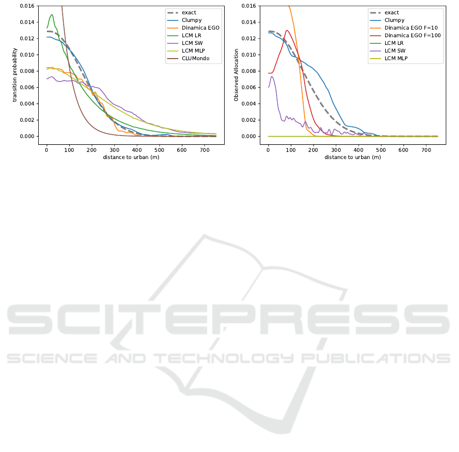
(a) Calibration-estimation comparison process. (b) Global calibration/allocation comparison process (for a
single allocation run).
Figure 2: Transition probability one-dimensional cut from agricultural to urban areas with respect to distance to existing urban
areas, with elevation set to 300 m and slope set to 2
o
.
of the calibration process, in comparison to exist-
ing calibration methods. We have also used a new,
bias-free, patch-allocation algorithm. This couple of
calibration-allocation procedures is always unbiased
and substantially more precise than existing ones. It
is more efficient in terms of computational time on
small (millions of pixels) problems, and significantly
faster (up to ∼ 100 times) than existing software on
large or very large problems (tens to hundreds of mil-
lions of pixels).
We have finally proposed an evaluation method
in section 4 allowing us to perform effective compar-
isons of the performances of various modeling envi-
ronments, including ours. This constitutes a first step
towards a systematic validation procedure for LULC
change models. This method takes advantage of the
fact that it is both more relevant and more efficient to
compare models in explanatory variable space rather
than in physical space. Indeed, LULC change cal-
ibration data are often undersampled, by necessity,
and the type of LULC change models analyzed here
is statistical in nature. Both features imply that try-
ing to reproduce transition locations exactly in phys-
ical space is often essentially impossible and mis-
leading. Instead, one should focus on reproducing
the correct probability structure in explanatory vari-
able space, and, to a lesser extent, in patch parame-
ter space (patch characteristics have not yet been seri-
ously characterized in existing LULC change model-
ing environments).
All these points will be elaborated upon in detail
in our forthcoming papers.
REFERENCES
Alexander, P., Prestele, R., Verburg, P. H., Arneth, A.,
Baranzelli, C., Batista e Silva, F., Brown, C., Butler,
A., Calvin, K., Dendoncker, N., Doelman, J. C., Dun-
ford, R., Engstr
¨
om, K., Eitelberg, D., Fujimori, S.,
Harrison, P. A., Hasegawa, T., Havlik, P., Holzhauer,
S., Humpen
¨
oder, F., Jacobs-Crisioni, C., Jain, A. K.,
Krisztin, T., Kyle, P., Lavalle, C., Lenton, T., Liu, J.,
Meiyappan, P., Popp, A., Powell, T., Sands, R. D.,
Schaldach, R., Stehfest, E., Steinbuks, J., Tabeau, A.,
van Meijl, H., Wise, M. A., and Rounsevell, M. D. A.
(2017). Assessing uncertainties in land cover projec-
tions. Global Change Biology, 23(2):767–781.
Chamayou, J. M. F. (1980). Averaging shifted histograms.
Computer Physics Communications, 21(2):145–161.
Charikar, M. and Siminelakis, P. (2017). Hashing-Based-
Estimators for Kernel Density in High Dimensions. In
2017 IEEE 58th Annual Symposium on Foundations of
Computer Science (FOCS), pages 1032–1043. ISSN:
0272-5428.
Eastman, J., Jin, W., Kyem, P., and Toledano, J. (1995).
Raster Procedure for Multi-Criteria/Multi-Objective
Decisions. Photogrammetric Engineering & Remote
Sensing, 61:539–547.
Garc
´
ıa-
´
Alvarez, D., Lloyd, C. D., Van Delden, H., and Ca-
macho Olmedo, M. T. (2019). Thematic resolution in-
fluence in spatial analysis. An application to Land Use
Cover Change (LUCC) modelling calibration. Com-
puters, Environment and Urban Systems, 78:101375.
Mas, J.-F., Kolb, M., Paegelow, M., Camacho Olmedo,
M. T., and Houet, T. (2014). Inductive pattern-based
land use/cover change models: A comparison of four
software packages. Environmental Modelling & Soft-
ware, 51:94–111.
O’Brien, T. A., Kashinath, K., Cavanaugh, N. R., Collins,
W. D., and O’Brien, J. P. (2016). A fast and objective
multidimensional kernel density estimation method:
A Formally Correct and Algorithmically Efficient LULC Change Model-building Environment
35

fastKDE. Computational Statistics & Data Analysis,
101:148–160.
Prestele, R., Alexander, P., Rounsevell, M. D. A., Arneth,
A., Calvin, K., Doelman, J., Eitelberg, D. A., En-
gstr
¨
om, K., Fujimori, S., Hasegawa, T., Havlik, P.,
Humpen
¨
oder, F., Jain, A. K., Krisztin, T., Kyle, P.,
Meiyappan, P., Popp, A., Sands, R. D., Schaldach, R.,
Sch
¨
ungel, J., Stehfest, E., Tabeau, A., Meijl, H. V.,
Vliet, J. V., and Verburg, P. H. (2016). Hotspots of
uncertainty in land-use and land-cover change pro-
jections: a global-scale model comparison. Global
Change Biology, 22(12):3967–3983.
Rudemo, M. (1982). Empirical Choice of Histograms and
Kernel Density Estimators. Scandinavian Journal of
Statistics, 9(2):65–78.
Sain, S. R., Baggerly, K. A., and Scott, D. W. (1994). Cross-
validation of multivariate densities. Journal of the
American Statistical Association, 89(427):807–817.
Scott, D. (2015). Multivariate density estimation: Theory,
practice, and visualization: Second edition. Wiley.
Soares-Filho, B. S., Coutinho Cerqueira, G., and
Lopes Pennachin, C. (2002). Dinamica — A stochas-
tic cellular automata model designed to simulate the
landscape dynamics in an Amazonian colonization
frontier. Ecological Modelling, 154(3):217–235.
Terrell, G. (1990). The Maximal Smoothing Principle in
Density Estimation. Journal of the American Statisti-
cal Association, 85(410):470–477.
van Vliet, J., Bregt, A. K., Brown, D. G., van Delden, H.,
Heckbert, S., and Verburg, P. H. (2016). A review
of current calibration and validation practices in land-
change modeling. Environmental Modelling & Soft-
ware, 82:174–182.
van Vliet, J., Malek, Z., and Verbug, P. (2015). The CLU-
Mondo land use change model, manual and exercises.
Vannier, C., Bierry, A., Longaretti, P.-Y., Nettier, B., Cor-
donnier, T., Chauvin, C., Bertrand, N., Qu
´
etier, F.,
Lasseur, R., and Lavorel, S. (2019a). Co-constructing
future land-use scenarios for the Grenoble region,
France. Landscape and Urban Planning, 190:103614.
Vannier, C., Lasseur, R., Crouzat, E., Byczek, C., Lafond,
V., Cordonnier, T., Longaretti, P.-Y., and Lavorel, S.
(2019b). Mapping ecosystem services bundles in a
heterogeneous mountain region. Ecosystems and Peo-
ple, 15:74–88.
Vannier, C., Lefebvre, J., Longaretti, P.-Y., and Lavorel, S.
(2016). Patterns of Landscape Change in a Rapidly
Urbanizing Mountain Region. Cybergeo.
Verburg, P. H., Alexander, P., Evans, T., Magliocca, N. R.,
Malek, Z., Rounsevell, M. D., and van Vliet, J. (2019).
Beyond land cover change: towards a new generation
of land use models. Current Opinion in Environmental
Sustainability, 38:77–85.
Verburg, P. H., de Koning, G. H. J., Kok, K., Veldkamp,
A., and Bouma, J. (1999). A spatial explicit allocation
procedure for modelling the pattern of land use change
based upon actual land use. Ecological Modelling,
116(1):45–61.
Wand, M. and Jones, C. (1994). Multivariate plug-in band-
width selection. Computational Statistics, 9(2):97–
116.
Wand, M. P. (1992). Error analysis for general multtvariate
kernel estimators. Journal of Nonparametric Statis-
tics, 2(1):1–15.
Wells, J. R. and Ting, K. M. (2019). A new simple and
efficient density estimator that enables fast systematic
search. Pattern Recognition Letters, 122:92–98.
APPENDIX
Case Study Transition Probability
Function
The parameters used to define the function P
∗
(v|u,y)
in Eq. (4) are the following:
µ = (150, 0,0) (5)
Σ =
25
2
843 325
843 10
2
−16.3
325 −16.3 10
2
(6)
D = {y | 0 ≤ y
0
≤ 616, 0 ≤ y
1
≤ 15, 0 ≤ y
2
≤ 60}
(7)
Models Parameters
In section 5, we use various land use change models
with the following parameters.
Dinamica EGO
We have used version 5.2.1 and all the calculations
were performed on a single CPU. The binning param-
eters are the following. The parameter increment is
fixed at 15 meters for the elevation, 5
o
for the slope
and 10 meters for the distance to urban areas. The
minimum delta, the maximum delta and the tolerance
angle are respectively fixed at 50, 500,000 and 5.0 for
all explanatory variables.
Idrisi LCM
We have an Idrisi Selva license, which is relatively old
(17.00). The estimation by logistic regression is done
without sampling. The parameters of SimWeight are
the default ones with notably the sample size fixed at
1000. All the default parameters of MLP are kept.
CLUMondo
We have used version 1.4.0. The sampling parameter
is fixed to 30% of all observations. The number of
cells distance between samples is fixed to 2 with no
data values excluding and balanced sample enabled.
Clumpy
The KDE parameter q (section 3.1.2) is fixed to 51.
This is the only user-defined parameter in CLUMPY.
This default value should be appropriate for most ap-
plications.
GISTAM 2022 - 8th International Conference on Geographical Information Systems Theory, Applications and Management
36
