
Results from using an Automl Tool for Error Analysis in
Manufacturing
Alexander Gerling
1,2,3
, Oliver Kamper
4
, Christian Seiffer
1
, Holger Ziekow
1
,
Ulf Schreier
1
, Andreas Hess
1
and Djaffar Ould Abdeslam
2,3
1
Business Information Systems, Furtwangen University of Applied Science, 78120 Furtwangen, Germany
2
IRIMAS Laboratory, Université de Haute-Alsace, 68100 Mulhouse, France
3
Université de Strasbourg, France
4
SICK AG, 79183 Waldkirch, Germany
{alexander.gerling, djaffar.ould-abdeslam}@uha.fr, oliver.kamper@sick.de
Keywords: AutoML Tool, Manufacturing, Production Line.
Abstract: Machine learning (ML) is increasingly used by various user groups to analyze product errors with data
recorded during production. Quality engineers and production engineers as well as data scientists are the main
users of ML in this area. Finding a product error is not a trivial task due to the complexity of today’s production
processes. Products have often many features to check and they are tested in various stages in the production
line. ML is a promising technology to analyze production errors. However, a key challenge for applying ML
in quality management is the usability of ML tools and the incorporation of domain knowledge for non-
experts. In this paper, we show results from using our AutoML tool for manufacturing. This tool makes the
use of domain knowledge in combination with ML easy to use for non-experts. We present findings obtained
with this approach along with five sample cases with different products and production lines. Within these
cases, we discuss the occurred error origins that were found and show the benefit of a supporting AutoML
tool.
1 INTRODUCTION
In recent years machine learning (ML) has been
progressively used in manufacturing to predict errors
(Li et al., 2019; Caggiano et al., 2019; Hirsch et al.,
2019). Modern explainable ML approaches open new
possibilities to analyze a product error. The objective
is to use ML as support to find the origin of a
production error. There are already data-driven
approaches for complex production systems (Ren et
al., 2020). Data‑driven quality prediction methods are
growing in various areas (Kirchen et al., 2019;
Tangjitsitcharoen and Ratanakuakangwan, 2017; Liu
et al., 2019a; Li et al., 2019), thanks to the rapid
development of artificial intelligence (AI) technology
and tools. Quality engineers are the main users to
analyze a product error in the manufacturing domain.
However, this is often not a trivial task, as there are
many test stations in today’s complex production
lines and products have a large number of features to
be tested. Also, quality engineers are often having
deep knowledge in the manufacturing domain but
have no expertise in data science techniques. This
impedes to the exploitation of ML potential in error
analysis. In (Wilhelm et al., 2020), we can find a brief
overview of problems and challenges of data science
approaches for quality control in manufacturing.
Further, we can find a description of the use of ML in
production lines in (Gerling et al., 2020).
As ML techniques and tools keep maturing, we
see the opportunity to combine data science
techniques with domain expert knowledge to create
applications for non-experts in the field of ML. The
aim is to make the use of ML accessible to quality
engineers. The key concept to enable this use of ML
for error analysis is Automated Machine Learning
(AutoML). AutoML is used to create an application
of ML, which is more feasible for a user and reduces
the required level of expertise. Examples for AutoML
solutions can be found in (Candel et al., 2016;
Golovin et al., 2017; Kotthoff et al., 2019; Feurer et
al., 2019). Within these solutions, we already benefit
from automating several steps of the data science
pipeline, like hyperparameter tuning of an algorithm.
100
Gerling, A., Kamper, O., Seiffer, C., Ziekow, H., Schreier, U., Hess, A. and Abdeslam, D.
Results from using an Automl Tool for Error Analysis in Manufacturing.
DOI: 10.5220/0010998100003179
In Proceedings of the 24th International Conference on Enterprise Information Systems (ICEIS 2022) - Volume 1, pages 100-111
ISBN: 978-989-758-569-2; ISSN: 2184-4992
Copyright
c
2022 by SCITEPRESS – Science and Technology Publications, Lda. All rights reserved
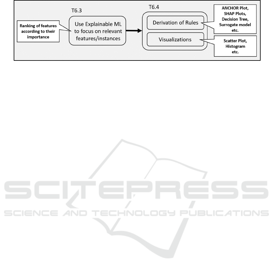
Figure 1: Cutout from Figure 7 (Seiffer et al., 2020).
One of the main tasks of a quality engineer is to
find faults in the production and eliminate them. This
task is very time-consuming and needs highly
specialized personnel, as a product often has many
features and is produced over several test stations.
Furthermore, an error could be caused by the
interaction of several features (e.g., overheating due
to current and voltage). A quality engineer must find
dependencies across several features, which is hardly
feasible for a human. Therefore, ML could be a great
help. To identify errors, we provide an AutoML tool
that creates various analyses and visualizations.
These are adjusted for the error analysis of a quality
engineer. The different types of visualizations can
further help to understand the error in-depth and get
more insights. Furthermore, automatic data analyses
can run along, which can indicate changes in
production. This can happen by an adjustment of the
production line or by the occurrence of a new error.
This information is particularly interesting, as it
contributes to detecting possible causes of errors
quickly.
In previous publications, we evaluated ML
techniques to reduce the dataset complexity, optimize
the results, or evaluated different visualizations for
the quality engineer. That is why, we want to
investigate in this paper if our ML tool provides the
important features for the analysis with the associated
visualizations which lead to the origin of the error.
Therefore, we would like to answer the following
research questions (RQ) through this paper:
• (RQ1) Can we provide important features for the
error analysis and derive target visualizations?
• (RQ2) Can a quality engineer find plausible
reasons for the errors?
The paper is organized as follows: Section 2
describes the potential of our AutoML tool. In Section
3 we provide an overview of similar applications or
approaches in production. The processing pipeline of
our AutoML tool is described in Section 4. We
discuss further information about domains
knowledge in Section 5. In Section 6 we describe five
investigated cases and the possible solutions for
identifying the error origin. We use Section 7 to
conclude our work.
2 USE CASE
With our AutoML tool PREFERML (Ziekow et al.,
2019b), we aim to support a quality engineer’s work.
The objective is that a quality engineer is able to work
autonomously without the help of a data scientist or
needs further ML knowledge to achieve results. We
accomplish this through the automation of processes
within our AutoML tool and the use of predefined
domain knowledge. Furthermore, our tool can be
integrated into the as-is process to reduce product
errors in the production line (Gerling et al., 2020) and
to support the quality engineer in his daily work.
We define the automated parts of our AutoML
tool by the Cross-Industry Standard Process for Data
Mining (CRISP-DM) (Chapman et al., 2000).
CRISP-DM has six phases, and we automate four of
them. That is, we use an extended notion of AutoML
which comprises the subsequent phases. (1) Data
Understanding: Here we model the provided domain
knowledge from the quality engineer for later use.
Therefore, we set the predefined key attributes for the
AutoML tool based on the product information. (2)
Data Preparation: In this phase, we prepare the data
with the help of the predefined domain knowledge, so
that the data could be used by the ML model. Within
this phase, missing or not usable values are
automatically removed. Also, the product data gets
enriched with derived features, by using the
information from the domain knowledge. Sometimes
an error is related to other product errors, and it is
beneficial to analyze them as a group. Therefore, our
AutoML tool has the possibility to group error
messages and analyze them as one product error. This
is especially useful if a product has detected several
similar faults in a test station. (3) Modeling: We
automate the feature selection and hyperparameter
tuning part to train the final ML model. (4)
Results from using an Automl Tool for Error Analysis in Manufacturing
101

Evaluation: In this phase, we provide selected and
adjusted visualizations and statistics for the user,
which is done automatically. Therefore, we improve
the automation of the analysis pipeline.
In our earlier work (Seiffer et al., 2020), we
describe a process to investigate errors using ML
support with a detailed explanation (see Figure 7 in
(Seiffer et al., 2020)). The process task is divided into
four subtasks. In Figure 1 we show a cutout from the
investigation process. Especially the displayed
subtasks T6.3 and T6.4 should be highlighted to
support the quality engineer in the automatic error
evaluation. Within these two tasks, we provide the
automatically necessary information and
visualizations for the analysis. In task T6.4 we
distinguish two possibilities for the deeper analysis.
(I) Derivation of Rules: this can be done by ML
agnostic tools, to explain the decisions of a model.
Well known libraries like ANCHOR (Ribeiro et al.,
2018), SHAP Plots (Lundberg and Lee, 2017) or a
Surrogate Model (Pedregosa et al., 2011) are used
here. Also, a decision tree from the model or a rule
list based on derived decision rules could be provided
(II) Visualizations: adjusted visualizations for the
quality engineer like Scatter Plots and Histograms are
used to get an overview over the distribution of the
measured product values. Further, a Correlation
Diagram can help to understand the correlation
between a feature and the test result.
3 RELATED WORK
In Dogan and Birant (Dogan and Birant, 2021), a
comprehensive literature review is provided for an
overview of how machine learning techniques can be
utilized to comprehend manufacturing mechanisms
with smart actions. The objective of this review was
to provide an understanding of the main approaches
and which algorithms were used to improve
manufacturing processes in the last years. They group
previous ML studies and the latest research in
manufacturing in four main subjects: monitoring,
quality, failure, and scheduling. Further, existing
solutions to various aspects of algorithms, tasks,
performance metrics, and learning types are provided
by Dogan and Birant. Also, an overview from
different perspectives about the current literature is
provided. The advantages of utilizing machine
learning techniques are provided and how to tackle
challenges for the manufacturing. Additionally,
further research directions in this area were provided.
In Turetskyy (Turetskyy et al., 2021), a battery
production design to use multi-output machine
learning models was provided. Lithium-ion battery
(LiB) cell manufacturing has high production costs
and a great impact on the environment. This is due to
the expensive materials, the high process fluctuations
with high scrap rates. Also, the energy demand for
this is especially high. Moreover, it is difficult to plan,
control and execute the production in this area
because of the lack of profound knowledge of LiB
cell production processes and their influence on the
quality. The multi-output approach is based on data-
driven models, which predict the final product
properties. This was done by the intermediate product
features. A concept was utilized in a case study within
the pilot line of the Battery LabFactory
Braunschweig. For the case study, 155 lithium-ion
battery cells were used to build an artificial neural
network model. The final product properties from
intermediate product features were later predicted by
the trained model. Within the provided concept, they
showed how the approach could be deployed within
the framework of a cyber-physical production system.
This is targeting for continuous improvement of the
underlying data-driven model and further, the
decision support in production.
In Liu (Liu et al., 2019b), a real-time quality
monitoring and diagnosis scheme for manufacturing
process profiles based on a deep belief network
(DBN) was developed. This is based on the ability of
DBN to extract the essential features from the input
data. This is essentially needed because the
manufacturing process has a large number of real-
time quality data, which are collected through various
sensors. Further, most of the data are high-dimension,
nonlinear and high-correlated. Therefore, it is
difficult to model the process profile, which limits the
function of a typical statistical process control
technique. They used the collected profile from a
manufacturing process and mapped it into quality
spectra. In this paper, a novel DBN recognition model
for quality spectra was established for the offline
learning phase. This can be used to monitor and
diagnose the process profiles in the online phase. To
test how effective the DBN recognition model for
manufacturing process profiles was, a simulation
experiment and a real injection molding process
example were used to analyze the performance. As
result, the proposed DBN model could outperform
alternative methods.
Soto, Tavakolizadeh, and Gyulai (Carvajal Soto et
al., 2019) present a machine learning and
orchestration framework for fault detection in
manufacturing. In the context of surface mount
devices, they propose a system for real-time machine
learning application. A key component of their work
ICEIS 2022 - 24th International Conference on Enterprise Information Systems
102

is the introduction of a discrete-event simulation that
allows failure detection approaches to be evaluated
without disrupting ongoing production operations.
The authors evaluate both random forests and
gradient boosting as alternatives for machine learning
algorithms. To avoid concept drift, ML models are
retrained at regular intervals. Both approaches show
convincing results in a case study. Their developed
approach fulfills the most important conditions of a
scalable, reconfigurable, adaptable, and re-
deployable solution. Scalability, acceptance,
however, have not been measured and generalization
and security still have to be proven.
In Olson and Moore (Olson and Moore, 2016), an
open-source genetic programming-based AutoML
system named TPOT is explained. This AutoML tool
automatically optimizes ML models and feature pre-
processors. An objective for the supervised
classification task is to optimize classification
accuracy. TPOT designs and optimizes the necessary
ML pipeline without any involvement of a human
being for a given problem domain (Olson et al.,
2016). TPOT uses a version of genetic programming
- an evolutionary computation technique to
accomplish this. It is possible to automatically create
computer programs (Banzhaf et al., 1998) with
genetic programming. For the supervised
classification, TPOT uses similar algorithms as we
do. However, our focus lies on tree-based algorithms
for understandable results, and we do not use e.g.,
logistic regression. After the usage of TPOT, the user
gets a file with code, which should help to execute the
ML process. In contrast, we do not deliver any files
with code but provide results with analyses and
supporting visualizations. Our AutoML tool further
provides a pre-processing and feature engineering
pipeline, which get automatically executed in the
process.
Maher and Sherif (Maher and Sakr, 2019) present
a meta learning-based framework for automated
selection and hyperparameter tuning for ML
algorithms (SmartML). The SmartML tool has a
meta-learning feature which mimics the role of a
domain expert in the area of ML. The meta learning
mechanism get used to select an algorithm to
minimize the parameter-tuning search space. Further,
the SmartML tool supply the user with a model
interpretability package to explain their results. In
contrast to SmartML, we pre-process the data with the
provided background information of a product. This
task could be done by a ML expert or a quality
engineer. Regarding the algorithm, we utilize a
decision tree-based algorithm to supply the user with
human recognizable and acceptable decisions. With
decision tree-based algorithms, we can improve the
confidence of the user in the given results. A main
distinction to SmartML is, that our tool is specialized
for the manufacturing domain. Highly unbalanced
data or the selection of a specific metric are not
supported by the SmartML tool.
Limits and possibilities of applying AutoML in
production are described by Krauß et al. (Krauß et al.,
2020). Their work provides an evaluation of available
systems. Further, it shows a comparison of a manual
implementation from data scientists and an AutoML
tool in a predictive quality use case. The result of this
comparison was that currently AutoML still requires
programming knowledge. Further, it was
outperformed by the implementation of the data
scientists. A critical point which led to this result was
the preparation of the needed data. For example, an
AutoML system cannot merge the data correctly
without predefined domain knowledge. Further, the
extraction from a database and the integration of the
data is problematic. An expert system could be the
solution for these problems. A further point was the
deployment of the results of the models. In summary,
it can be said that the AutoML system delivers a
chance to improve the efficiency of an ML project.
This could be achieved by automating the necessary
procedure within Data Preparation, Data Integration,
Modelling, and Deployment. Domain knowledge and
the expertise of a data scientist should be included in
this to obtain satisfying results. However, the newest
developments show evidence for upcoming
improvements towards the automation of specific
steps within the ML pipeline.
Our work represents an AutoML approach for
manufacturing that is aided by domain knowledge.
This helps to automate the ML pipeline and further
can narrow the error root cause analysis. With the
AutoML approach, data scientists are able to perform
error-oriented analyses without prior knowledge in
the field of ML. Further, feature importance statics
are providing hints to the important feature
visualizations, which are automatically created.
4 PROCESSING PIPELINE
In this section, we discuss the workflow of our
AutoML tool and the processing pipeline. The first
step is to merge the data from various test stations.
From the domain knowledge, we can derive the order
of the test stations and merge the data. As the next
step, we read and clean the data e.g., from missing
values. The next step is to prepare the data by
removing unnecessary features e.g., features with
Results from using an Automl Tool for Error Analysis in Manufacturing
103

only one value in the column and check the data
format. In the following step, we use domain
knowledge to create the derived features. Afterwards,
we split the data in a predefined percentage split into
a train and test set. The test set always contains 33%
of the errors from the dataset. The next step is the
training and optimization of the ML model. We use
the XGBoost classifier (eXtreme gradient boosting)
(Chen and Guestrin, 2016) as its ML core, as we value
comprehensibility in our model higher than
prediction accuracy. The optimization is performed
on a cost-based metric that maximizes business value.
To optimize the model training, the user can select
hyperparameter tuning and feature selection
separately or together if the user wants to improve the
model performance further. Feature selection is a
valid method to reduce the complexity of data and
reduces the search space for the error origin.
Therefore, feature selection can be used for the
analysis. Even if the users cannot achieve a better
result but can reduce the complexity of the data, they
can benefit from the reduction of features. After using
the feature selection method, only the most relevant
features for the model are left. Feature selection
requires time and computation power which varies
depending on the dimensionality of the dataset. Our
tool can perform feature selection strategies in
different ways (Gerling et al., 2021b).
Hyperparameter tuning of the model is a method
to optimize the model even more and benefit from
better results. However, hyperparameter tuning is not
a universal solution to improve the results and uses a
lot of computation resources. We are evaluating
possibilities to use highly parallel computation
methods to reduce the time needed for this step.
Next, we evaluate the results and check the
created visualizations. We create multiple adjusted
visualizations for the error root cause analysis for the
quality engineer. For example, a scatter plot can be
used to see in which value area an error appears and
if there are changes in the measured values over time.
Moreover, the scatter plot shows indirect the timeline
of the production and when a product error has
appeared. An evaluation of possible visualization to
use for the production can be found in (Gerling al.,
2021a). For the evaluation, we check the model
performance based on our cost-based metric. Based
on the model performance, we can identify beneficial
trained models. Here, a good-performing model can
indicate the origin of an error and can help to save
costs. We check the feature importance of each
feature. To do so, we use various model-dependent
and independent feature importance techniques e.g.,
total gain, gain, and SHAP Max Main Effect (Ziekow
et al., 2019a). Also, we check the correlation between
each feature and the test result with the Kendall's tau
correlation (Virtanen et al., 2020). Based on the
importance order of the features, we check
sequentially the created visualizations of each. A
further possibility to analysis the product error and to
inspect the decision from the model are provided by
a decision tree. The XGBoost classifier uses multiple
decision trees within the boosting approach.
Therefore, we use a surrogate model to provide the
approximate decision rules from the model
represented by one decision tree. The decision rules
from the trained model can be further derived and
directly be used in form of a rule list. This can be done
by providing the associated rules for the analysis.
To start it is advisable to let the PREFERML
AutoML tool run through the complete process
without making any additional settings like activating
feature selection. Therefore, we use the standard
parameter settings for the initial process run. These
initial results may already highlight features that are
correlated to the error. Within the provided results,
the user can check the given statistics of the results
and features that were weighted most strongly by the
ML model. The benefit of this initial process is, that
feasible results can already be quickly achieved with
this procedure and bring insights into the origin of an
error.
5 DOMAIN KNOWLEDGE
The domain knowledge of a product is represented as
a simple ontology. An illustration of the ontology can
be found in (Gerling et al., 2020). To create the
ontology, the quality engineer is the most suitable
user. The ontology has pre-defined key attributes
from a product. The key attributes include
information about the product, test stations (Test
System), test specification, and production line.
Every test station in a production line can be defined
separately in the ontology and thus offers variable
adaptation options. For example, the user configures
the sequence of test stations and further necessary
information about the product. The ontology -
respectively a representation of the domain
knowledge - is crucial to automate the ML tool.
During the execution of a process, the defined key
attributes are accessed within the ontology and used
for specific process execution. One of the key
attributes is the name of the previous test station.
With this information, we can derive the order of the
test stations in the production line. Moreover, we can
derive and determine a unique product feature to track
ICEIS 2022 - 24th International Conference on Enterprise Information Systems
104
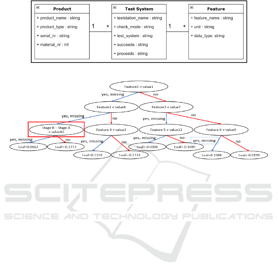
Figure 2: Simplified ontology (presented as entity relationship model).
Figure 3: Decision tree.
products across several test stations. With both
mentioned information, our tool can merge data from
various test stations and use it later for the analysis.
Further features to be defined are datetime and
categorical features. From the datetime feature, we
can derive time-relevant features. The categorical
features will be converted into usable information for
the classifier. Soon, we will extend information of a
future by additional information like the unit i.e., volt
or ampere. With this additional information, further
derivations can be carried out. Moreover, features
with similar units can be grouped and selected or
removed for later analyses. This allows a specific
error to be narrowed down even further and simplifies
the analysis.
In Figure 2 we illustrate a simplified UML
diagram for the ontology for our AutoML tool. We
show how the three classes are connected and their
specific attributes. In the Test System class, we have
the attributes succeeds and proceeds, which helps to
rebuild the production line structure. This represents
the Test System and Production Line from our
ontology (Gerling et al., 2020). In the Product class,
we have the attributes serial_nr and material_nr.
These two attributes may be combined and could
represent one value/attribute to create a unique
identifier. However, there may be cases in which
more than two features or even just one can serve as
a unique identifier. In the Feature class we can use the
unit attribute to afterwards create feature groups from
the production data. The unit attribute could
especially be used to narrow down the origin of an
error. The Feature class represents the Test
Specification from our ontology.
6 RESULTS
In this section, we show five specific cases from five
different products. We discuss the reasons for the
production error and show visualizations from our
AutoML tool which help to identify them. To protect
the confidential information of our partner company,
we only visualize important features with obfuscated
values and names.
6.1 Case 1
In the first case, we analyzed the general error
probability in four consecutive production steps. The
production setup for this product is already highly
optimized, so no quick results could be found by the
quality engineers anymore. Also, most of the features
that could possibly correlate to any common error
were investigated before. In this situation, quality
engineers approached us with the need to further
reduce the generally low error probability. This is
why we did not focus on a specific error.
Results from using an Automl Tool for Error Analysis in Manufacturing
105

We could achieve a good result for error
prediction but - at the first glance - no clear
correlation between the errors with any specific
feature could be identified. However, a naive
approach of analyzing the first decision tree of the
XGBoost model, a user with domain knowledge
background was able to identify a specific feature. In
Figure 3 we can see the first decision tree of the model
and at the lower-left corner the identified feature. This
visualization is automatically created by our AutoML
tool and shows the rules that are used by the ML
Model. Moreover, a decision tree shows multiple
chains of rules that can be utilized for independent
error analysis. In this case, the feature identified by a
quality engineer was generated during data
preprocessing and was not part of the initial dataset.
This shows why good feature engineering can
significantly improve the results and create insights
that are hard to achieve by a human.
Figure 4: Time difference stage B – stage A.
As the next step, we took a closer look at the
histogram of the time difference feature. In Figure 4
we can see that this error held further hidden
information. On the x-axis of the histogram, the value
range is divided into several buckets which represent
the number of days. The columns are colored darker
depending on the percentage of corrupt products. As
an aid, the number of absolute and the percentage of
corrupt products within the separated value range is
shown above the column. The y-axis shows the
number of instances in a natural logarithm to provide
a better visual representation. In this figure, we can
recognize that the percentage of corrupt parts is
significantly too high if the time difference is smaller
than 5 hours. This means that the product must rest
longer between to stations to reduce the number of
errors.
After a discussion with the quality engineer, we
found that the product parts are treated with glue at
the first station. This means, that we possibly
identified the error root cause and are now evaluating
a rule to let the product rest longer between the
stations. The results of this evaluation are still
pending. In this specific case, the time difference was
not the origin of the error but provided a direct hint.
By identifying this feature, a quality engineer was
able to perform more in-depth and targeted analyses.
6.2 Case 2
In the second case, we analyzed the specific error
message “Measurement Accuracy Distance Value too
high”. This error cause could be found through
analyzing the feature importance. Based on the
feature importance, the “Material number” was the
most important feature.
Figure 5: Error frequency depending on material number.
In Figure 5 we can see that all errors correspond
to the value range of 15 to 18 of the material number.
As the material number corresponds to a certain type
of subproduct, we can specify further analyses with
these. It has turned out that the subproduct types with
the material number 15 - 18 have different
specifications regarding range and accuracy.
Figure 6: Measurement accuracy maximum distance
value 1.
Figure 6 shows the second most important feature
for this case. The device accuracy is measured on
different targets (e.g., reflectors or 5%-black) in
different distances ranging from very close to very
far. Measurement 1 is done on a reflecting foil in a
ICEIS 2022 - 24th International Conference on Enterprise Information Systems
106
very close range, so the detector is near its saturation.
Measuring with too high accuracy here leads to bad
results in long range measurements on less reflective
targets. It might very well be, that the device is
electrically overcompensating, or emitter and
detector are not adjusted in a perfect manner.
Nearly all occurred errors are in the value range
of approximately 27-29. Whereas good parts range
from 64 to 68 approx. This information can further
strengthen the analysis of the product error and lead
us to a specific feature respectively product part. We
suggested that, as a first step, all product parts that are
unique to the material numbers 15+ and that may
influence the accuracy of the measurements to be
investigated further.
6.3 Case 3
In our third case, we analyze another product error, in
which we did not optimize the model for one specific
error but for a general error prediction. We retrieved
data from a chain of test stations from a production
line. The following visualizations belong to a specific
test station. In this case, the most important feature
was the modulation feature. Modulation is the process
of adding information to an electrical or optical
carrier signal. The modulation can change the signal’s
frequency (frequency modulation, FM) or its
amplitude (amplitude modulation, AM). In Figure 7
we can see this feature and the increasing error rate in
the higher value range.
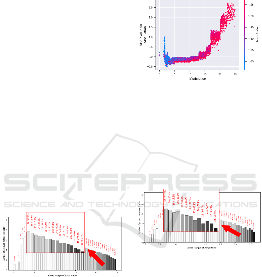
Figure 7: Error frequency depending on modulation.
We further create a SHAP dependence plot
(Lundberg and Lee, 2017) for the modulation feature
in Figure 8.
At the x-axis the modulation feature with the
value range. On the left side of the y-axis, we see the
associated SHAP value for the modulation feature.
The right side of the y-axis shows the feature with the
highest interaction with the modulation feature and
the associated values of this feature. High feature
values are colored in red and low feature values are
Figure 8: Modulation SHAP dependence plot.
colored in blue. Therefore, we know that the
modulation feature has the most interaction with the
amplitude feature, which is also the second most
important feature by the feature importance. The error
probability (high SHAP value) is increased with an
increasing value of modulation. Furthermore, an
interaction between modulation and amplitude can be
seen. A high modulation value goes together with a
high amplitude value. This correlation between
modulation and amplitude is already known by a
quality engineer but the provided visualization
strengthens the trust in our AutoML tool because it
shows the real behavior of product features.
Figure 9: Error frequency depending on amplitude.
Next, the amplitude feature is shown in Figure 9.
This feature was the second most important based on
the feature importance list. This visualization shows
that products with a high amplitude tend to make
errors more often. If technically possible and
economically rational, it might be a good idea to
switch from amplitude to frequency modulation,
which is a lot more robust against amplitude changes
of the base signal.
Based on Figure 8 and Figure 9 it became clear
that a solution correcting the root cause will not be
achieved quickly. In the meantime, one could
implement a control function within the testing
equipment to detect error-prone combinations of the
mentioned features. Modules with high amplitudes
Results from using an Automl Tool for Error Analysis in Manufacturing
107
and / or modulation could be sorted out in the
production line as early as possible. Even if the error
will not disappear completely in this case, the
situation will improve as our tool is optimizing the
model towards an economic optimum and not 0%
error rate.
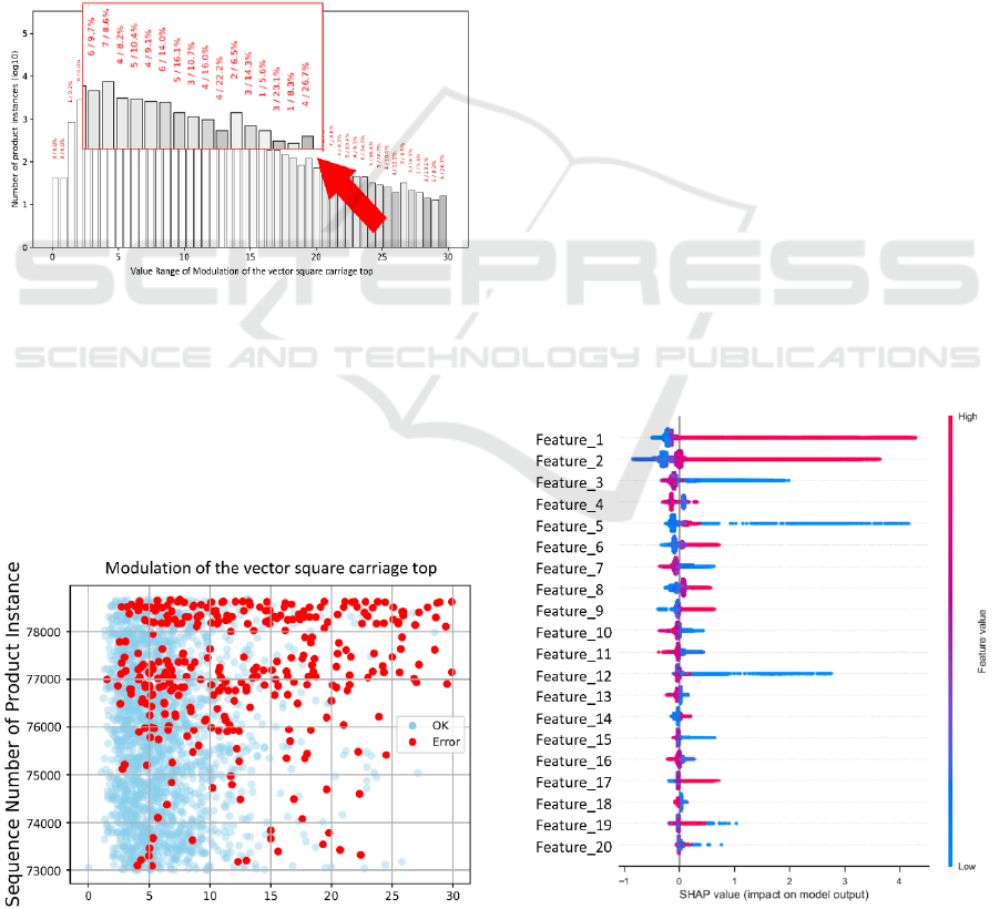
6.4 Case 4
For the fourth case, we analyze the specific product
error “Cosine trace too high”. In this case, we took
features from one test station to predict errors at the
subsequent test station in the production line. The
most important feature here is “vector square carriage
top”. We first take a look at the histogram of this
feature in Figure 10.
Figure 10: Modulation of vector square carriage top.
We can see that the highest error probability is
related to the value of the feature ranging from 21 to
29. Here we could restrict the tolerance or only let
through products with the maximum value of 20. At
first glance, this amount of error might be acceptable
if the error is not extremely expensive. However, in
this case we want to show another relevant factor in
manufacturing.
Figure 11: Modulation of the vector square carriage top
scatter plot.
In Figure 11 we show the time progression of the
error as it occurred. In this visualization, the latest
products are represented by a high product instance
number. It can be seen that the error caused by this
feature has occurred in two waves and was relevant at
the time of analysis. Note, that not all good products
are shown in this visualization to reduce overplotting.
Specifically, we randomly selected 2000 data points
of good products and visualized them alongside all
errors that occurred. Nevertheless, due to the actuality
of the occurred errors, we could consult with the
responsible employees about recent changes in the
production. This could create further conclusion of
the occurred product error. Through this discussion, a
solution to the error could be found and as a
consequence, the production could be corrected. We
suggested to investigate the change before the start of
the second wave of errors and the change that led to
the end of the first wave.
6.5 Case 5
In this case, we want to highlight the advantage to use
model agnostic techniques within our AutoML tool.
These techniques help to comprehend the model
decisions and provide an additional way to analyze
the error cause further. We take advantage of this to
automatically provide customized visualizations for
the user. For this purpose, we show two visualizations
that demonstrate the learned decision of the trained
ML model. For the sake of demonstration, we
obfuscated the feature names and values.
Figure 12: SHAP summary plot.
ICEIS 2022 - 24th International Conference on Enterprise Information Systems
108
For a deeper investigation of the origin of an
error, a SHAP Summary Plot (Lundberg and Lee,
2017) is automatically generated by our AutoML
tool. Here, the features learned from the model are
sorted from top to bottom in order of feature
importance. With this plot, we can visualize various
information to the quality engineer. First, the
importance of the features and their order. Further,
the different dots are colored according to the value
of each instance. Moreover, the SHAP value on the x-
axis shows a tendency if a product instance could be
good (negative SHAP value) or corrupted (positive
SHAP value). In Figure 12 we can see that Feature_1
and Feature_2 both tend to an error when the
measured value is high with a SHAP value over 3.
Also, feature Feature_3, Feature_5, and Feature_12
tend to an error when the measured value is low.
Feature_5 represents a time difference between two
test stations, which was derived with the help of
domain knowledge. As can be seen in the SHAP
Summary Plot, the product has a higher tendency to
fail when the value is low. For the explanation, at test
station A a heat test was performed on a product.
After that, the product was cooled down in the
subsequent test station B. If the internal components
of the product are still too hot, this product will not
pass the followed check at test station B. In a further
investigation, we saw that the product should
approximately cool down about 8 minutes, or else the
ratio to fail the test station check at test station B will
be much higher.
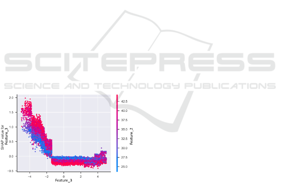
Figure 13: SHAP dependence plot of Feature_3.
In Figure 13 we show the SHAP Dependence Plot
of Feature_3 from the previous visualization. We
found the strongest interaction between Feature_3
and Feature_2. In this visualization, we can see in-
depth, how the values of this feature are distributed in
three distinguishable regions. One region spanning
from values of -4.5 to approx. -1.8 and another one in
range of approx. -1.8 to approx. 5.0. It should be
investigated what the cause for this behavior is
especially in the last region of values in the range
from -4.0 to -4.5 where a high SHAP values are given.
6.6 Lessons Learned
With the above-described cases, we demonstrated the
benefit to use our AutoML tool. First, we can support
the tasks of a quality engineer with meaningful
visualizations and further information about the error
root cause analysis. This speeds up the time between
the error’s first occurrence and the implementation of
a solution.
We provide further visualization technics with the
help of ML-like in the test case. A further advantage
is, that a quality engineer can use our tool without any
knowledge in the field of ML while at the same time
the data scientist does not need specific domain
knowledge because this can be easily formalized and
provided in a single file by the quality engineer. By
automating the data merging, processing, and
enhancement, we save the quality engineer time and
bring helpful information to the analysis like the time
differences between test stations. The user is provided
with the most important features for the analysis,
which often lead to the origin of an error.
Furthermore, the visualized feature can point to
hidden causes of errors like in Case 1. Therefore, it is
important to include as much relevant data for
analysis as possible. Often, even trivial reasons such
as the temperature in the production hall or the time
of production can bring decisive advantages to the
analysis.
7 CONCLUSION
In this paper, we investigate the benefit of AutoML
for error analysis in manufacturing along with real-
world cases. We describe the difficulties that arise in
a complex production environment and provide a
brief overview of the workflow. In five real-world use
cases, we could provide respectively assist in
identifying the error origin using AutoML. In these
five cases, we found clear correlations to a possible
error origin. Further, we provide domain experts the
possibility to combine domain knowledge of a
product or production line with an easy-to-use
AutoML tool. This leads to a synergy that would
otherwise be unused. Therefore, we offer a data
science layperson the possibility, without prior
knowledge in the field of ML, to use our AutoML tool
and benefit from the advantages for an analysis.
Results from using an Automl Tool for Error Analysis in Manufacturing
109

Through this paper, we now can answer the
research questions from the introduction. First, we
demonstrated that the PREFERML AutoML tool
provided useful visualization and further information
to analyze the origin of an error (RQ1). Even if a
visualization could not show the direct cause of an
error, it could point out an important feature that led
to a possible reason, as in case 1 (RQ2). Furthermore,
we found that, if the root cause was not found or could
not be solved, our tool gives easy guidelines on how
to implement a function or process to sort out
products with a high error probability.
In the near future, we want to use domain
knowledge more efficiently by establishing an
advantage product ontology. Further, we want to test
our AutoML tool with more products and gather
feedback from different user groups to improve it
even more. We also want to improve the Explainable
ML part of the AutoML tool to provide further
analysis to quality engineers and support the ML
decision with various visualizations.
ACKNOWLEDGEMENTS
This project was funded by the German Federal
Ministry of Education and Research, funding line
“Forschung an Fachhochschulen mit Unternehmen
(FHProfUnt)“, contract number 13FH249PX6. The
responsibility for the content of this publication lies
with the authors. Also, we want to thank the company
SICK AG for the cooperation and partial funding.
REFERENCES
Banzhaf, W., Nordin, P., Keller, R. E., and Francone, F. D.
1998. Genetic programming: an introduction: on the
automatic evolution of computer programs and its
applications. Morgan Kaufmann Publishers Inc.
Caggiano, A., Zhang, J., Alfieri, V., Caiazzo, F., Gao, R.,
and Teti, R. 2019. Machine learning-based image
processing for on-line defect recognition in additive
manufacturing. CIRP Annals 68, 1, 451–454.
Candel, A., Parmar, V., LeDell, E., and Arora, A. 2016.
Deep learning with H2O. H2O. ai Inc, 1–21.
Carvajal Soto, J. A., Tavakolizadeh, F., and Gyulai, D.
2019. An online machine learning framework for early
detection of product failures in an Industry 4.0 context.
International Journal of Computer Integrated
Manufacturing 32, 4-5, 452–465.
Chapman, P., Clinton, J., Kerber, R., Khabaza, T., Reinartz,
T., Shearer, C., Wirth, R., and others. 2000. CRISP-DM
1.0: Step-by-step data mining guide. SPSS inc 9, 13.
Chen, T., & Guestrin, C. (2016). XGBoost: A Scalable Tree
Boosting System. In Proceedings of the 22nd ACM
SIGKDD International Conference on Knowledge
Discovery and Data Mining (pp. 785–794). New York,
NY, USA: ACM.
https://doi.org/10.1145/2939672.2939785
Dogan, A. and Birant, D. 2021. Machine learning and data
mining in manufacturing. Expert Systems with
Applications 166, 114060.
Feurer, M., Klein, A., Eggensperger, K., Springenberg, J.
T., Blum, M., and Hutter, F. 2019. Auto-sklearn:
efficient and robust automated machine learning. In
Automated Machine Learning. Springer, Cham, 113–
134.
Gerling, A., Schreier, U., Heß, A., Saleh, A., Ziekow, H.,
Abdeslam, D. O., Nandzik, J., Hannemann, J., Flores-
Herr, N., and Bossert, K. 2020. A Reference Process
Model for Machine Learning Aided Production Quality
Management. In ICEIS (1), 515–523.
Gerling, A., Seiffer, C., Ziekow, H., Schreier, U., Hess, A.
and Abdeslam, D. 2021a. Evaluation of Visualization
Concepts for Explainable Machine Learning Methods
in the Context of Manufacturing. In Proceedings of the
5th International Conference on Computer-Human
Interaction Research and Applications, pages 189-201.
Gerling, A., Ziekow, H., Schreier, U., Seiffer, C., Hess, A.,
and Abdeslam, D. O. 2021b. Evaluation of Filter
Methods for Feature Selection by Using Real
Manufacturing Data. In DATA ANALYTICS 2021:
The Tenth International Conference on Data Analytics,
October 3-7, 2021, Barcelona, Spain, 82–91.
Golovin, D., Solnik, B., Moitra, S., Kochanski, G., Karro,
J., and Sculley, D. 2017. Google vizier: A service for
black-box optimization. In Proceedings of the 23rd
ACM SIGKDD international conference on knowledge
discovery and data mining, 1487–1495.
Hirsch, V., Reimann, P., and Mitschang, B. 2019. Data-
driven fault diagnosis in end-of-line testing of complex
products. In 2019 IEEE International Conference on
Data Science and Advanced Analytics (DSAA), 492–
503.
Kirchen, I., Vogel-Heuser, B., Hildenbrand, P., Schulte, R.,
Vogel, M., Lechner, M., and Merklein, M. 2017. Data-
driven model development for quality prediction in
forming technology. In 2017 IEEE 15th international
conference on industrial informatics (INDIN), 775–
780.
Krauß, J., B. M. Pacheco, H. M. Zang, and R. H. Schmitt.
“Automated Machine Learning for Predictive Quality
in Production.” Procedia CIRP 93 (2020): 443–48.
https://doi.org/https://doi.org/10.1016/j.procir.2020.04.
039.
Kotthoff, L., Thornton, C., Hoos, H. H., Hutter, F., and
Leyton-Brown, K. 2019. Auto-WEKA: Automatic
model selection and hyperparameter optimization in
WEKA. In Automated Machine Learning. Springer,
Cham, 81–95.
Li, Z., Zhang, Z., Shi, J., and Wu, D. 2019. Prediction of
surface roughness in extrusion-based additive
ICEIS 2022 - 24th International Conference on Enterprise Information Systems
110

manufacturing with machine learning. Robotics and
Computer-Integrated Manufacturing 57, 488–495.
Liu, G., Gao, X., You, D., and Zhang, N. 2019a. Prediction
of high power laser welding status based on PCA and
SVM classification of multiple sensors. Journal of
Intelligent Manufacturing 30, 2, 821–832.
Liu, Y., Zhou, H., Tsung, F., and Zhang, S. 2019b. Real-
time quality monitoring and diagnosis for
manufacturing process profiles based on deep belief
networks. Computers & Industrial Engineering 136,
494–503.
Lundberg, S., & Lee, S. I. (2017). A unified approach to
interpreting model predictions. arXiv preprint
arXiv:1705.07874.
Maher, Mohamed Mohamed Maher Zenhom Abdelrahman,
and Sherif Sakr. 2019. SmartML: A Meta Learning-
Based Framework for Automated Selection and
Hyperparameter Tuning for Machine Learning
Algorithms. EDBT: 22nd International Conference on
Extending Database Technology, Mar.,
doi:10.5441/002/edbt.2019.54.
Olson, R. S. and Moore, J. H. 2016. TPOT: A tree-based
pipeline optimization tool for automating machine
learning. In Workshop on automatic machine learning,
66–74.
Olson, R. S., Urbanowicz, R. J., Andrews, P. C., Lavender,
N. A., La Kidd, C., and Moore, J. H. 2016. Automating
biomedical data science through tree-based pipeline
optimization. In European conference on the
applications of evolutionary computation, 123–137.
Pedregosa, F., Varoquaux, G., Gramfort, A., Michel, V.,
Thirion, B., Grisel, O., Blondel, M., Prettenhofer, P.,
Weiss, R., Dubourg, V., Vanderplas, J., Passos, D.,
Brucher, M., Perrot, M., & Duchesnay, E. (2011).
Scikit-learn: Machine Learning in Python. Journal of
Machine Learning Research, 12, 2825–2830.Ribeiro,
M. T., Singh, S., & Guestrin, C. (2016). "Why
Should I Trust You?". Proceedings of the 22nd ACM
SIGKDD International Conference on Knowledge
Discovery and Data Mining.
https://doi.org/10.1145/2939672.2939778
Ren, L., Meng, Z., Wang, X., Zhang, L., and Yang, L. T.
2020. A data-driven approach of product quality
prediction for complex production systems. IEEE
Transactions on Industrial Informatics.
Seiffer, C., Gerling, A., Schreier, U., & Ziekow, H. 2020.
A Reference Process and Domain Model for Machine
Learning Based Production Fault Analysis. In
International Conference on Enterprise Information
Systems (pp. 140-157). Springer, Cham.
Seiffer, C., Ziekow, H., Schreier, U., and Gerling, A. 2021.
Detection of Concept Drift in Manufacturing Data with
SHAP Values to Improve Error Prediction. In DATA
ANALYTICS 2021: The Tenth International
Conference on Data Analytics, October 3-7, 2021,
Barcelona, Spain, 51–60.
Tangjitsitcharoen, S., Thesniyom, P., and
Ratanakuakangwan, S. 2017. Prediction of surface
roughness in ball-end milling process by utilizing
dynamic cutting force ratio. Journal of Intelligent
Manufacturing 28, 1, 13–21.
Turetskyy, A., Wessel, J., Herrmann, C., and Thiede, S.
2021. Battery production design using multi-output
machine learning models. Energy Storage Materials 38,
93–112.
Virtanen, Pauli; Gommers, Ralf; Oliphant, Travis E.;
Haberland, Matt; Reddy, Tyler; Cournapeau, David et
al. (2020): SciPy 1.0: Fundamental Algorithms for
Scientific Computing in Python. In: Nature Methods
17, S. 261–272. DOI: 10.1038/s41592-019-0686-2.
Wilhelm, Y., Schreier, U., Reimann, P., Mitschang, B., and
Ziekow, H. 2020. Data Science Approaches to Quality
Control in Manufacturing: A Review of Problems,
Challenges and Architecture. In Symposium and
Summer School on Service-Oriented Computing, 45–
65.
Ziekow, H., Schreier, U., Gerling, A., & Saleh, A. 2019a.
Technical Report: Interpretable machine learning for
quality engineering in manufacturing-Importance
measures that reveal insights on errors.
Ziekow, H., Schreier, U., Saleh, A., Rudolph, C., Ketterer,
K., Grozinger, D., and Gerling, A. 2019b. Proactive
error prevention in manufacturing based on an
adaptable machine learning environment. In Artificial
Intelligence: From Research to Application: Proc. of
the Upper-Rhine Artificial Intelligence Symposium
UR-AI, 113–117.
Results from using an Automl Tool for Error Analysis in Manufacturing
111
