A Robust Modiﬁed Hybrid A*-based Closed-loop Local Trajectory

Planner for Complex Dynamic Environments

Chinnawut Nantabut

and Dirk Abel

Institute of Automatic Control, RWTH Aachen University, Campus Boulevard 30, Aachen 52074, Germany

Keywords:

Collision Avoidance, Autonomous Driving, Path Planning, Trajectory Planning, Object Detection, L-Shape

Fitting, Hybrid A*, Weighted A*, Stanley Controller, PID Controller, Bicycle Reciprocal Collision Avoidance.

Abstract:

In the research ﬁeld of autonomous driving, planning safe and effective trajectories is a key issue, which

also requires reliable detection of objects in the environment. This publication introduces a new approach to

compute safe trajectories for automated road vehicles quickly and robustly, also considering reliable object

detection for static and dynamic objects. For this purpose, the Hybrid A* algorithm modiﬁed with Weighted

A* is used to accelerate the planning of a collision-free path because the weight w can make the heuristic

term h become more important and make the tree much more narrow in the direction of the goal. Afterwards,

PID- as well as Stanley controllers are utilized to realize reliable trajectories. This combined algorithm is

extended with the L-Shape ﬁtting algorithm to detect objects in the environment. The entire approach is

evaluated for unstructured and semistructured environments using simulations of an automated vehicle with

a realistic interaction of dynamic obstacles in the presence of model and sensor uncertainties, guarantees a

real-time capability of 1 s, and results in collision-free vehicle movement. The whole algorithm, which yields

very promising results, will be transferred to a C++ framework and tested with ﬂexible test vehicles in real

environments in the future.

1 INTRODUCTION

Many companies and research institutions are en-

gaged in the realization of autonomous driving, which

is very challenging because the autonomous system

must perform all functions from planning and imple-

menting driving functions to system monitoring and

emergency management. In order to avoid any col-

lision in any case, it is essential that the system has

an exact scene understanding of the static environ-

ment and the complex behavior of dynamic obstacles.

The resulting trajectories, which the system calculates

based on the current trafﬁc situation, must be adjusted

permanently in real time by means of a closed con-

trol loop. Normally, path or trajectory planning ap-

proaches are validated only for structured (infrastruc-

ture is previously known), unstructured environment

(obstacles are detected online) or semistructured (the

combination of both cases). In our case, we consider

both types of environments where obstacles have to

be detected and the replanning is oftentimes activated

when needed. Furthermore, we take into account the

https://orcid.org/0000-0002-5767-6023

https://orcid.org/0000-0003-0286-3654

interactions of all trafﬁc participants for more realistic

test scenarios. Recently, researchers are mainly de-

veloping methods to tackle the following problems:

scene understanding, trajectory planning and trajec-

tory control. The implemented methods then perform

well either in complex dynamic environments, which

must be permanently observed, or in structured envi-

ronments, whose layout may already be known in ad-

vance. In most scientiﬁc work, dynamic obstacles are

considered challenging due to their poorly predictable

behavior, but the movement must still be considered

at all times. Most works in literature focus only on

the planning of collision-free paths that can simply

be driven using a feedforward controller which does

not continuously prove if the desired behavior is ac-

tually reached or not. If dealing with collision avoid-

ance, many papers describe non-convex optimization

problems to deal with unstructured and cluttered en-

vironments. But the calculated path is probably local

minimal or it is quite time-consuming due to the non-

convex search space. In order to be more speciﬁc and

to identify development needs, an overview of rele-

vant scientiﬁc work is given next.

Nantabut, C. and Abel, D.

A Robust Modiﬁed Hybrid A*-based Closed-loop Local Trajectory Planner for Complex Dynamic Environments.

DOI: 10.5220/0010997800003191

In Proceedings of the 8th International Conference on Vehicle Technology and Intelligent Transport Systems (VEHITS 2022), pages 26-35

ISBN: 978-989-758-573-9; ISSN: 2184-495X

The path planning method can be categorized into

graph-based and sample-based methods (Paden et al.,

2016), (Gonz

alez et al., 2016). Other approaches use

neural networks or stochastic methods, e.g., evolu-

tional strategies and can be combined with conven-

tional methods to optimize the results (Patle et al.,

2019). For the graph-based approaches, Dijkstra or

A* algorithms are applicable for the problems that

are deﬁned by a grid-based formulation. For exam-

ple, the continuous search space is partitioned into

a discrete one deﬁned by a grid. The search space

is not inﬁnitely large anymore and, therefore, facil-

itates the searching algorithm for ﬁnding a suitable

path. Unfortunately, there is no guarantee of ﬁnd-

ing an optimal path if not enough calculation time is

provided. A*, however, does not perform well in dy-

namically changing environments because it recalcu-

lates the path always from start point to end point in

each time step. That means the method is quite com-

putationally intensive, especially when the dimension

of the search space is high. D* has been developed

then, which is able to correct the calculated path con-

sidering new obstacles on the way. Both algorithms,

still, do not consider the realistic motion behavior of

vehicles where the path to be followed is curvy. To

address this challenge, Hybrid A* ﬁrst demonstrated

its successful usage on the Stanford Racing Teams

robot in the DARPA Urban Challenge in 2007 (Dol-

gov et al., 2008). They tested the implementation on

the simulated environments such as labyrinths, park-

ing lots and U-turns. A real-time Hybrid A* was

successfully implemented and evaluated for the KTH

Research concept vehicle using Dubins curve for for-

ward driving (Dolgov et al., 2010). The cost func-

tion used for smoothing a path in Hybrid A* was ex-

tended by considering the lane network of the park-

ing lot for semistructure application by combining the

topological graph search and the free-space path plan-

ning to reduce the number of expanded nodes (Kurzer,

2016). The three papers above, however, updated the

environments using SLAM as an input for the ex-

act path planning, which comes with high computa-

tional costs. Hybrid A* was applied to solve the path

planning problem in structured environments contain-

ing streets and in unstructured environments for non-

holonomous vehicles (Petereit et al., 2012). The out-

standing feature of this approach is the smooth visit

of a series of given waypoints. The obstacles were,

however, predeﬁned and the experimental part only

observed one speciﬁc example. To increase the per-

formance of the algorithm, the visibility graph was

used for the given polygonal obstacle’s vertices to

ﬁnd the optimal waypoints of the holonomic path up

to the goal region, which helps dramatically reduce

the number of expanding nodes. Here, the obstacle

conﬁguration and the available map were pre-deﬁned

as well (Sedighi et al., 2019). Hybrid A* was then

applied for unstructured environments, whereas state

lattice veriﬁcation technique has switched to struc-

tured applications (Guirguis et al., 2019). The method

was successfully tested in simulations for lane follow-

ing tasks, but not for a cluttered environment. the

Hybrid A* was optimized for wheeled robots in con-

sideration of a collision risk with dynamic obstacles

(Nemec et al., 2019). The overall calculation time

was limited to 1 s so that the real-time capability of

the path planning was guaranteed. However, the ob-

stacles are also predeﬁned and it is actually not clear

if the weight helps accelerate ﬁnding the path.

In the papers mentioned above, the obstacle recog-

nition part normally utilizes the occupancy grid map-

ping. However, this uses the full information of the

obstacle conﬁguration is not necessary when we can

assume almost all of the obstacles are rectangular as

in the parking lot or street scenarios. Therefore, Hy-

brid A* as a local planner in combination with model-

based, i.e. using the geometry information, object de-

tection seems promising but has not received much

attention in any research study until now.

To acquire an accurate detection of the environ-

ment, multiple sensors, such as LiDAR, radars, and

cameras, are used in this paper combined with the

well-known L-Shape approach to detect other vehi-

cles in the vicinity. In our approach, unstructured en-

vironments are considered, for which the Hybrid A*

approach has proven to be very promising. It calcu-

lates a path using discrete steering angle values and

a kinematic model of the ego-vehicle in a discrete

search space containing position and orientation. Fur-

thermore, Weighted A*, an algorithm to accelerate

the search with a suboptimal solution, is combined,

which seems suitable for unstructured and semistruc-

tured environments. The interaction of dynamic ob-

stacles, here vehicles, is implemented using the bi-

cycle reciprocal collision avoidance method (Alonso-

Mora et al., 2012). The trajectory control is then real-

ized by applying a PID controller for velocity control

along the path and a Stanley controller for keeping the

vehicle on the track laterally.

The paper furthermore focuses on the detection

and the decision-making modules. Detected objects

can be fed into the decision-making module directly

where path and trajectory planning take place. The

decision maker performs a calculation of the path

parameterized by time to realize the trajectory plan-

ning. One hundred scenarios for each unstructured

and semistructured environment are randomly gener-

ated to validate the robustness of the approach.

A Robust Modiﬁed Hybrid A*-based Closed-loop Local Trajectory Planner for Complex Dynamic Environments

The approach introduced in this paper calculates

collision-free trajectories in all situations while keep-

ing the calculation time under 1 s for real-time ap-

plications. However, this assumption is valid in the

simulation when using the search algorithm because

collisions can still occur in reality, especially in the

high-speed networks as on highways. The work is

therefore applicable for the case of low-speed range

(< 10 m/s) as in parking lots.

2 METHOD

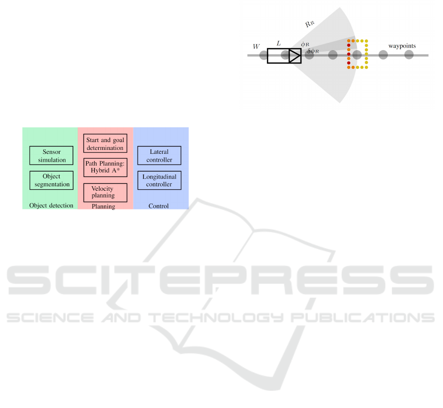
Figure 1: A workﬂow of the trajectory planning demon-

strated in this work is presented.

At ﬁrst, the position, the orientation, the size as well

as the velocity of an ego vehicle is previously known.

A reference path is given for the vehicle to follow and

no obstacles are present. The vehicle tracks on this

given path as long as no obstacles are detected. If

that is not the case, a collision avoidance framework

presented in this paper is activated and a collision-free

path and a desired velocity are then calculated. Figure

1 summarizes the entire work consisting of three main

modules. Obstacles are deﬁned previously, detected

and then segmented in the simulation by the sensor

of an autonomous vehicle at every time step. During

the object detection step, LiDAR data is continuously

processed using an L-Shape ﬁtting approach to gen-

erate suitable rectangular bounding boxes for all ob-

stacles in sight. The bounding boxes are then fed to

the trajectory planning consisting of a planning and

velocity planning part. In the planning module, the

start and goal points are reasonably determined for

ﬁnding a new path using Hybrid A* in combination

of Weighted A* algorithm, in dependence on the type

of environments. They have to be far enough all of

the obstacle points for the sake of the collision avoid-

ance. The path planning algorithm is activated in case

that the obstacles stay in the way. The velocity plan-

ner then uses the distance to the next front object to

ﬁnd a desired or reference velocity. The controllers

hereinafter are activated to keep the vehicle on track.

2.1 Object Detection: Sensor

Simulation

Figure 2: The points detected by the LiDAR sensor attached

on a vehicle of length L and width W are simulated.

Figure 2 illustrates how to simulate a LiDAR sensor

used in the experiments in the paper. A previously de-

ﬁned path for the ego vehicle is given by a set of gray

circular waypoints. The detection range of the sen-

sor is provided by a gray circular arc on the black ego

vehicle. A static obstacle depicted in yellow points

is deﬁned beforehand in the simulation. The orange

points are the ones that lying within the sensor range

and the red points are the real ones that will be pre-

processed in the object segmentation module.

The waypoints deﬁning the path can be deter-

mined ofﬂine by using the previously known informa-

tion with a ﬁxed goal point by, for example, a conven-

tional A* algorithm. Otherwise, the path can be just

deﬁned by a center line of the lane in case that the ve-

hicle just follows a lane in case of a route planning.

In this paper, however, the waypoints are given and

the ego vehicle tries to track the resulting path while

keep itself away from collision with the surrounding

obstacles detected online.

Supposingly, the yellow rectangular obstacle’s

points representing both static such as vehicles stand-

ing still in a parking lot or the driving ones are prede-

ﬁned pointwise. The orange points within the sensor

range of radius R

and angle ϕ

are considered. Only

one red point of each circular segment of angle δϕ

is regarded for the calculation in the upcoming part to

optimize the calculation time. All of these detected

points are then submitted to the preprocessor in order

to calculate the possible rectangular conﬁguration of

the obstacles deﬁned by 4 vertices for each at that mo-

ment. If at least one of the obstacle’s points is stand-

ing within the range around the predeﬁned path, the

path planning and the control module of the frame-

work are then activated so that the ego vehicle can

avoid serious collisions.

VEHITS 2022 - 8th International Conference on Vehicle Technology and Intelligent Transport Systems

2.2 Object Detection: Object

Segmentation

L-Shape ﬁtting is a model-based vehicle detection and

tracking used under the assumption that rectangle ob-

stacles are detected from the side by the laser scanner

in the form of L (Zhang et al., 2017) . The procedure

generates a sample of rotated boxes for each segment

of the point cloud and then compares them to deter-

mine which one best suits all of the points using a

minimal distance criterion. These points are the red

ones that we obtained from the procedure that we just

explained earlier.

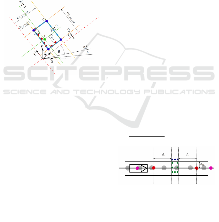
Figure 3: An L-Shape ﬁtting algorithm is utilized for the

detection of a rectangular obstacle.

Figure 3 demonstrates how the L-Shape ﬁtting al-

gorithm works. One of the clusters of the prepro-

cessed point cloud, in red, from the previous sensor

simulation in Figure 2 is processed in this step, re-

sulting in the blue bounding box with the dark blue

vertices. Each green point i from this cluster is con-

sidered for comparing the distance to the bounding

box.

The coordinate system (x, y) is ﬁxed at the sensor.

The rotated coordinate system (x

, y

) which suits the

obstacle best is to be determined. The algorithm deals

with the combinatorial least square problem described

by searching for the two perpendicular line equations

and choose which line each point of the cluster be-

longs to. Out of three criteria, the closeness maxi-

mization is utilized because of the good average time

consumption and exactness of detection (Zhang et al.,

2017). This criterion ﬁnds the conﬁguration of the ro-

tated box the sum of which of the distance of the red

points to their closest side of the box is minimal.

Instead of directly solving the least-square prob-

lem, a brute force search is carried out to reduce the

calculation time by deﬁning a search angle increment

θ = nδ, where n ∈Z

∪{0}and 0 6 θ <

. The calcu-

lation for each angle can be done parallely to improve

the real-time capability and the solution is acceptable

when the angular resolution δ is small enough. The

corresponding perpendicular line equations for point

i (green from Figure 3.) at this angle are

cos(θ) + y

sin(θ) = c

1,i

(1)

and

−x

sin(θ) + y

cos(θ) = c

2,i

. (2)

1,i

and c

2,i

are the distances of point i to the ro-

tated coordinate system which can be compared to

ﬁnd the boundary of the box. This is deﬁned by

the line equations with c

1,min

= minc

1,i

and c

1,max

maxc

1,i

for the ﬁrst equation and c

2,min

= min c

2,i

and c

2,max

= max c

2,i

for the second equation. The

minimal distance of this point to the bounding box

i,min

= min(min(c

1,i

−c

1,min

, c

1,max

−c

1,i

), min(c

2,i

−

2,min

, c

2,max

−c

2,i

)) is calculated and the sum of this

minimal distance of each point S

∑

i,min

quanti-

ﬁes how well the current box matches the cluster. The

box at the angle of θ

min

with the smallest sum is cho-

sen. The matrix L summarizes all the coefﬁcients of

the lines plus a repetition of the ﬁrst line to determine

the four vertices.

L = [l

i, j

]

5×3







cos(θ

min

) sin(θ

min

) c

1,min

−sin(θ

min

) cos(θ

min

) c

2,min

cos(θ

min

) sin(θ

min

) c

1,max

−sin(θ

min

) cos(θ

min

) c

2,max

cos(θ

min

) sin(θ

min

) c

1,min







(3)

The vertex v

(blue) of each box with i ∈

{1, 2, 3, 4} is calculated by using the element of the

matrix L as follows,

i,1

i+1,2

−l

i,2

i+1,1



i,3

i+1,2

−l

i,2

i+1,3

i,1

i+1,3

−l

i,3

i+1,1



(4)

Figure 4: The start and goal conﬁgurations for determining

a collision-free path by Hybrid A* are differently chosen in

dependence of the environment types.

These four vertices of each segment are then sent

to the path planning module for the collision avoid-

ance to determine the start and goal conﬁguration us-

ing in the path planning algorithm.

A Robust Modiﬁed Hybrid A*-based Closed-loop Local Trajectory Planner for Complex Dynamic Environments

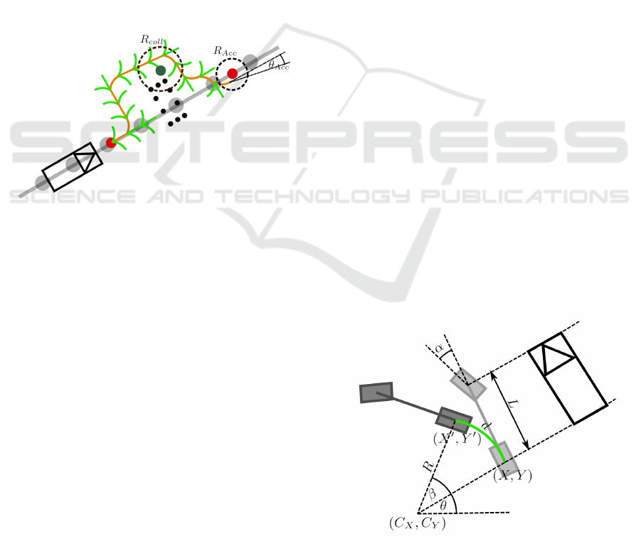
Figure 4 explains how to determine start and goal

points needed for the path planning algorithm. The

points for the unstructured environments are por-

trayed in pink, while the ones for the semistructured

scenarios in red. Obstacles’ points that could lead to

potential collision danger to the vehicle are depicted

in green, while those in the safer zones are illustrated

in blue.

In case of unstructured environments, the start

point can be easily deﬁned as the current position

and the goal point can be the end of the given path.

For semistructured cases, however, the vehicle has to

stay within the street as long as possible. All obsta-

cle points within range d

are projected to the orig-

inal path. Let d

, the safe distance from the closest

projected obstacle point, ﬁrst equal to d

, the safe dis-

tance from the most distant projected obstacle point.

If the start point goes behind the vehicle, we then set

the start point to the current position and orientation

of this vehicle.

Figure 5: Tree expansion of the Hybrid A* algorithm is ap-

plied in order to determine an optimal collision-free path

for a nonholonomic vehicle. The tree is not expanded in

the vicinity of the obstacles and the expansion process is

stopped when the last node is in the goal area with an ac-

ceptable orientation deviation.

2.3 Planning: Path Planning with

Modiﬁed Hybrid A*

Hybrid A* calculates, in comparison to A*, a smooth

path comprising a set of small smooth paths from one

state to another, depicted in Figure 5 (Dolgov et al.,

2008). It uses the red start and goal conﬁguration to

ﬁnd a collision-free path based on the expansion of

the green tree starting incrementally from the current

node to its neighboring nodes and so on. As a result,

an orange optimal path is calculated.

The algorithm compares the approximated length

f of the path via each neighboring node and chooses

the most promising one with the least f . This term

can be expressed as

f = g + wh, (5)

where g is the exact path length from the start to that

neighboring node, h is the approximated path length

from the neighboring node to the goal node which

can be a heuristic and w is the weight to accelerate

the search with the greedy behavior to the goal point

which is normally used in Weighted A*.

By expanding the tree, the dark green node cannot

be added if it is too close to the obstacle points within

the range of R

coll

. The tree expansion is stopped when

the successor node is within the radius of R

Acc

and

the deviation of the orientation is within θ

Acc

. The

optimal path is then traced back from the goal to the

start node.

The original Hybrid A* algorithm employs two

admissible heuristics to ﬁnd the most promising suc-

cessor (Dolgov et al., 2008), (Dolgov et al., 2010).

That means the heuristics h are not larger than the real

path length from the current to the goal node so that

the search algorithm is applicable.

The ﬁrst heuristic considers the nonholonomity of

the vehicle without taking into account the obstacles

in the environments. It uses motion primitives which

can be seen as a set of short paths that can be reused in

every node expansion step by rotating in accordance

with the orientation of the current node. The inputs

of each motion primitive, i.e. the control input and

the vehicle model parameters, stay the same until the

next node is reached. Dubins or Reeds-Shepp curves

are used to accelerate the tree expansion.

The second heuristic, on the contrary, regards the

environments, but not the kinematic model of the ve-

hicle or the smoothness of the path. It uses the ”ﬂow

ﬁeld” when multiple start points are given for a cer-

tain goal point (Emerson, 2019). This can be applied

as well for the Voronoi ﬁeld. This determines which

grid cell of the search space belongs to which obstacle

by using the obstacle itself as the start point.

Figure 6: The motion primitive is calculated for the tree

expansion by using the single track model for Hybrid A* as

explained in Equations (6)-(8) (Udacity, 2015).

VEHITS 2022 - 8th International Conference on Vehicle Technology and Intelligent Transport Systems

Instead of expanding the successors around the

current node into the next cells as in A*, Hybrid A*

uses the kinematic model to expand the tree for the

ﬁrst heuristic as shown in Figure 6. Hereby, the black

vehicle is transformed into a single track model de-

picted as a ”bicycle” in gray. The new state of the

vehicle is illustrated as the black bicycle after travers-

ing the green path with a distance of length d.

The algorithm discretizes the control variables,

such as the steering angle, and determines the suc-

cessor nodes with the help of single track model for

nonholonomic vehicles. The model assumes that the

wheels of each axis are shifted to the longitudinal axis

of the vehicle and the center of mass to the ground to

reduce the degrees of freedom of the model and facil-

itate the calculation of the successor nodes depicted

in gray.

To determine the motion primitive, the algorithm

calculates ﬁrst the driving angle β given the driv-

ing distance d which is the length of the diago-

nal of the cell plus an offset so that the successor

node can locate in the neighboring grid cell, wheel

base L and the steering angle α from the set of

{−α

max

, ..., 0, ..., +α

max

}, with the vehicle projected

to a single track model:

β =

tan(α). (6)

The radius R of the motion is then calculated and

used for determining the center of the circular motion

R =

. (7)

The angle from the turning center to the rear wheel

center θ in return is used for calculating the successor

node (X

)







−R sin(θ) + R sin(θ + β)

+ R cos(θ) + R cos(θ + β)



(8)

To limit the calculation time, the maximal itera-

tion is set to N

I,max

, each with the maximal steering

angle α

max

and n

discrete values. The tree can then

be expanded by a Dubins curve to link the node which

yields the smallest f value and the goal point. Dubins

curve use the start and end conﬁguration, calculate the

path lengths of 6 possible movements when available,

and compare them to ﬁnd the shortest path. Further-

more, we do not consider the obstacle, since practi-

cally, we still do not know how the obstacle conﬁg-

uration looks like when it is located further from the

current position. We then expand the tree from the

node that has the largest approximated cost f because

the path that ends with this node is found with the

exactness of path length quantiﬁed by f . The approx-

imated remaining path length from the Hybrid A*’s

end node to the goal point, or h, can be determined

by the simple geometry of Dubins or Reed-Shepps

curves.

Figure 7: A path calculated by the tree expansion is opti-

mized in view of four criteria.

J = w

∑

i=1

, y

) + w

∑

i=1

(|x

−o

|−d

max

)

N−1

∑

i=1

(

∆φ

|∆x

−κ

max

) + w

N−1

∑

i=1

(∆x

x+1

−∆x

)

(9)

The cost function J from Equation 9 is illustrated

in Figure 7 (Dolgov et al., 2008). It optimizes the cal-

culate path in orange, deﬁned by N way points con-

siders the Voronoi ﬁeld value σ

(=0 in Voronoi edges

(pink) and =1 next to and in obstacles) the distance

to the nearest obstacle | x

−o

| compared to max-

imal allowed distance (light blue) d

max

, the actual

curvature

∆φ

|∆x

compared to maximal allowed curva-

ture κ

max

and the vector change to the neighboring

nodes of node i. The last two terms use the infor-

mation about the current and both consecutive points

(green). The two terms in the middle are quadratic

penalties. The points are then updated by conjugate

gradient optimization (CG), which can be easily im-

plemented (Shewchuk, 1994). An oversampling of

nodes is carried out by placing one more point be-

tween two consecutive segments and re-optimized by

using the same optimization techniques.

Due to the fact that Hybrid A* rarely yields the

path that leads to the exact continuous goal conﬁgu-

ration, the end of the tree is set to the predeﬁned goal

conﬁguration.

2.4 Planning: Velocity Planning

In Figure 8, the controllers for both longitudinal and

lateral direction are illustrated. The desired longitudi-

A Robust Modiﬁed Hybrid A*-based Closed-loop Local Trajectory Planner for Complex Dynamic Environments

nal velocity of the ego v

lon

depends on the current dis-

tance d

from the front axis of the ego vehicle along

the path to the nearest next vehicle within the range

of d

. The desired velocity proﬁle can be deﬁned in

three sections by introducing two offsets d

x,1

and d

x,2

When the distance d

is less than d

x,1

, the vehicle tries

to stop and therefore v

lon,desired

. In the second ﬁeld,

the desired velocity v

lon,desired

rises linearly with the

current distance d

. After the offset d

x,2

, the desired

velocity is kept constant according to the ego’s vehi-

cle desired velocity.

Figure 8: A PID controller is utilized for the longitudinal

speed control and a Stanley controller for the lateral control.

2.5 Control: Longitudinal and Lateral

Controller

As mentioned earlier, two controllers are employed,

which are illustrated in Figure 8. A PID controller

is applied for regulating the vehicle’s longitudinal ve-

locity v

lon

to be as close to v

lon,desired

as possible. The

smaller its value is, the less velocity the ego vehicle

desires to have. To eliminate the deviation of the lat-

eral distance to the path e

and the deviation of the

orientation ∆θ, a Stanley controller is utilized (Thrun

et al., 2006).

3 VALIDATION

We evaluate the performance of the modiﬁed Hybrid

A* in a combination of L-Shape ﬁtting object de-

tection in the simulations for both unstructured and

semistructured environments in the presence of dy-

namic obstacles.

3.1 Simulation Setup

The implementation of Hybrid A* is based on the

open-source C# implementation (Nordeus, 2015).

However, we decided to reimplement it in MATLAB.

There are many reasons for this. Firstly, we can carry

on an analysis of the algorithm through implementing

on our own and can develope it for the future by com-

bining Hybrid A* with more algorithms from the A*

family such as Dynamic A*, Anytime Repairing A*

or even Anytime Dynamic A*. Secondly, although

MATLAB also provides a Navigation Toolbox com-

prising of Hybrid A* path planning, we cannot mod-

ify the weight inﬂating the heuristic as used in this

paper. Lastly, we will transfer the implemented MAT-

LAB code onto a Simulink Real-Time target used in

a host computer on our model vehicle ”Buggy” de-

veloped by our institute (Reiter et al., 2017). We use

Dubins curve instead to consider only forward move-

ments. If the Reed-Shepps curves were implemented,

which is normally used in Hybrid A*, the behavior of

node expansion would still be similar. The maximal

iteration n

I,max

for tree expansion is set to 10. The

maximal steering angle α

max

is set to 45 deg to make

the vehicle only drive forward and n

= 5 discrete

values. The driving distance d is set to

√

2 + 0.01

m, which is the diagonal length of each grid cell (cell

size is 1 m long) plus some offset to make sure the

successor node lies in another grid. The wheel base

of all vehicles L is 2 m. In addition, all weights w

of the cost function J for the optimization are set to

one for simplicity in order to equally consider all of

the components of the cost function. The weights are

needed to be tuned using machine learning methods

in the future.

We investigate the use of the modiﬁed Hybrid A*

in two types of environments as always mentioned.

The search space of size 20 m × 20 m is ﬁlled with

previously known rectangular obstacles. The two ex-

periments handle the unstructured and semistructured

environments of grid size 20 m × 20 m for a full tra-

jectory planning which consider both obstacle detec-

tion and control steps.

Figure 9 summarizes the interaction of the ego

vehicle and the obstacles in the unstructured and

semistructured environments. Hereby, the static ob-

stacles x

ob j

(green) are available for all trafﬁc partic-

ipants. We assume that all dynamic obstacles (red)

have full knowledge of the conﬁguration of static ob-

stacles x

ob j

. Meanwhile, the ego vehicle (blue) can

only receive partial information of static obstacles

due to the equipped sensor and can be described by

sensor



ob j



Furthermore, to model the vehicle’s interaction,

these pieces of information of another dynamic ob-

stacles are exchanged among themselves. The bicy-

cle reciprocal collision avoidance method (B-ORCA)

is utilized due to the fact that it considers the non-

VEHITS 2022 - 8th International Conference on Vehicle Technology and Intelligent Transport Systems

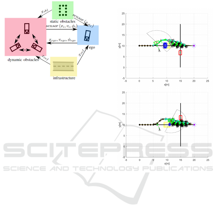
Figure 9: We test the modiﬁed Hybrid A* in both environ-

ments in the presence of static and dynamic obstacles. The

infrastructure is activated in addition for the semistructure

scenarios.

holonomic conditions of vehicles based on optimal re-

ciprocal collision avoidance (ORCA) (Alonso-Mora

et al., 2012). The vehicles interact properly to the

other vehicles which act differently, which is useful

in our case since one of the trafﬁc participants, here

an ego vehicle, is equipped with the modiﬁed Hybrid

A* to guide its behaviour. The responsibility factor

of each dynamic obstacle to another one or to the ego

vehicle is set to 0.5 since each vehicle tries to avoid

each other or taking half of the responsibilities. The

static obstacles, on the other hand, cannot move itself

and thus have no responsibility to avoid other trafﬁc

participants. The responsibility factor is then set to 0,

while all vehicles take full responsibility (the factor

equals 1).

Here as well, the vehicles have the full knowl-

edge of another dynamic obstacles’ conﬁguration

, v

, φ

and the ego’s position, velocity and orienta-

tion, x

ego

, v

ego

, φ

ego

. Meanwhile, due to the equipped

sensor, the ego vehicle can only collect partial infor-

mation described by sensor (x

, v

, φ

On top of that, The infrastructure part (yellow) is

deactivated for the second case, i.e. the unstructured

environment. In this use case, the infrastructure can

be constructed as a road deﬁned by two parallel point-

wised static obstacles with one side of length zero.

Since the infrastructure is previously known, its full

information x

in f

can be sent to all vehicles in the last

use case.

For both cases, the robustness of the modiﬁed Hy-

brid A* is evaluated by 100 random simulations each.

In the case of semistructured environment, we addi-

tionally deﬁne road boundaries with a lane width of 2

m each. Static obstacles are placed within the road,

while the vehicles try to follow their assigned lane.

3.2 Simulation Results

Figure 10: Application of the modiﬁed Hybrid A* as a local

planer in an unstructured environment: In the ﬁrst part of

the ﬁgure, the ego vehicle plans the new path to avoid the

collision with the static obstacle. As soon as the dynamic

obstacle is detected, a new path is calculated as well, as in

the second part of the ﬁgure.

In Figure 10, one of the testing scenarios for an un-

structured environment is evaluated. The green ego

vehicle moves to the right, while the red obstacle ve-

hicle progresses upwards. Their predeﬁned straight

paths are marked as black lines. As explained ear-

lier for the unstructured case, the start point in red

star falls upon the current position of the ego vehicle,

while the goal point in blue star corresponds to the

last waypoint of the track. A yellow rectangular static

obstacle is placed in the middle of the path. The blue

points are result of the L-Shaped ﬁtting algorithm and

display a current potential danger on track for the ego

vehicle. The black branches of the tree illustrate all of

the possible route, while the green leaves demonstrate

the potential nodes within the closed list of the Hybrid

A* algorithm. At ﬁrst, the ego vehicle is shifted to the

left side of the predeﬁned path to see whether the lat-

eral displacement is later compensated by the Stanley

A Robust Modiﬁed Hybrid A*-based Closed-loop Local Trajectory Planner for Complex Dynamic Environments

Figure 11: Application of the modiﬁed Hybrid A* as a local

planer in an semistructured environment. The scenario is

divided into two parts as in Figure 10. The road boundaries

are, however, previously known and constrain the free space

for the tree expansion.

controller. When the static obstacle is located within

the sensor range, the detected points are checked if

they could be seen dangerous to the vehicle by cal-

culating their distance to the tracked path. When the

obstacle hinders the movement of the ego vehicle, the

points detected by the sensor are feeded into the ob-

ject detection path to calculate the current obstacle

conﬁguration using L-Shape ﬁtting. A new path is

calculated using the modiﬁed Hybrid A* so that the

vehicle can avoid the currently detected obstacle. The

tree is expanded from start to goal points lying in the

original path. The new path is then followed using

Stanley controller while trying to keep its desired ve-

locity using an underlying PID controller. Once the

other vehicle is detected, the ego vehicle slows down

as in Figure below. However, another new path is cal-

culated so that the ego vehicle does not have to wait

until the dynamic obstacle ﬁnally leaves the danger-

ous zone. Afterwards, the ego vehicle speeds up to its

preferred speed and reach the original black path.

Figure 11 illustrates a collision avoidance for the

semistructured case by adding boundaries of the road,

marked as black dotted lines. Other illustrating el-

ements are the same as in Figure 10. Furthermore,

since the search space is limited, the procedure of

ﬁnding the path until the ﬁxed end point in large blue

star is facilitated in comparison to the previous case.

The lila waypoints illustrates the path joining the end

point of the planning and the end of the street. An

obstacle vehicle in this case drives in another lane in

opposite direction. It is clear that the tree only ex-

pands inside of these lane boundaries. As soon as the

ego vehicle detects the moving obstacle, it replans the

path and moves to the original lane as we can see from

Figure 11.

We test for robustness by randomly placing vehi-

cles and obstacles in both unstructured and semistruc-

tured environments. As a result, the ego vehicle can

safely avoid the collision with all the obstacles in all

of the simulation scenarios within the required time

for real-time capability of 1 s. This time limit is the

maximal time to be accepted in the real-time capabil-

ity in the guidance of autonomous vehicles and can

be reduced by improving the implementated code or

moving to the more efﬁcient platform such as Robot

Operating System(ROS). Furthermore, the inertia of

the vehicle is omitted which plays an essential role

in the dynamics and will be considered in the future

work.

4 CONCLUSIONS

We investigate the use of the modiﬁed Hybrid A* on

the robustness in unstructured and semistructured en-

vironments with a more realistic interaction of the

trafﬁc participants. The approach, combined with

the model-based L-Shape ﬁtting object detection, the

Stanley controller for lateral and PID controller for

longitudinal control, successfully ﬁnds the collision-

free path in the simulation with the presence of both

static and dynamic obstacles. The vehicle can ro-

bustly avoid collision within less than 1 s in the guid-

ance of autonomous vehicles.

In future works, we are going to validate quantita-

tively, in both simulations and experiments with ran-

dom conﬁgurations, the calculated path and to opti-

mize the weights of the cost function of Hybrid A*

for a better result of the path planned in both un-

structured and semistructured environments. The al-

gorithm will be tested in both Simulink-based model

using xPC Target and be transferred to a C++-based

ROS environment in the test vehicle for a real-time ca-

pability comparison. A more robust object detection

VEHITS 2022 - 8th International Conference on Vehicle Technology and Intelligent Transport Systems

algorithm can also be used for a more precise locali-

sation of the obstacles for a more robust path planning

in the real application.

ACKNOWLEDGEMENTS

The ﬁrst author would like to express attitude to-

wards National Science and Technology Develop-

ment Agency (NSTDA) for the ﬁnancial support dur-

ing the doctoral study in Germany as well as towards

the second author for the supervision in the doctoral

study.

REFERENCES

Alonso-Mora, J., Breitenmoser, A., Beardsley, P., and Sieg-

wart, R. (2012). Reciprocal collision avoidance for

multiple car-like robots. Proceedings - IEEE Interna-

tional Conference on Robotics and Automation, pages

360–366.

Dolgov, D., Thrun, S., Montemerlo, M., and Diebel, J.

(2008). Practical search techniques in path planning

for autonomous driving. In Proceedings of the First

International Symposium on Search Techniques in Ar-

tiﬁcial Intelligence and Robotics (STAIR-08).

Dolgov, D., Thrun, S., Montemerlo, M., and Diebel, J.

(2010). Path planning for autonomous vehicles in

unknown semi-structured environments. The Interna-

tional Journal of Robotics Research, 29(5):485–501.

Emerson, E. (2019). Crowd pathﬁnding and steering using

ﬂow ﬁeld tiles. Game AI Pro 360.

Gonz

alez, D., P

erez, J., Milan

es, V., and Nashashibi, F.

(2016). A review of motion planning techniques for

automated vehicles. IEEE Transactions on Intelligent

Transportation Systems, 17(4):1135–1145.

Guirguis, S. E., Gergis, M., Elias, C. M., Shehata, O. M.,

and Abdennadher, S. (2019). Ros-based model pre-

dictive trajectory tracking control architecture using

lidar-based mapping and hybrid a* planning. 2019

IEEE Intelligent Transportation Systems Conference

(ITSC), pages 2750–2756.

Kurzer, K. (2016). Path Planning in Unstructured Envi-

ronments: A Real-time Hybrid A* Implementation for

Fast and Deterministic Path Generation for the KTH

Research Concept Vehicle. PhD thesis.

Nemec, D., Gregor, M., Buben

ıkov

a, E., Hrubo

s, M.,

and Pirn

ık, R. (2019). Improving the hybrid a*

method for a non-holonomic wheeled robot. In-

ternational Journal of Advanced Robotic Systems,

16(1):1729881419826857.

Nordeus, E. (2015). Explaining the hybrid a star

pathﬁnding algorithm for selfdriving cars.

https://blog.habrador.com/2015/11/explaining-

hybrid-star-pathﬁnding.html.

Paden, B., C

ap, M., Yong, S. Z., Yershov, D. S., and Fraz-

zoli, E. (2016). A survey of motion planning and con-

trol techniques for self-driving urban vehicles. CoRR,

abs/1604.07446.

Patle, B., Babu L, G., Pandey, A., Parhi, D., and Jagadeesh,

A. (2019). A review: On path planning strategies

for navigation of mobile robot. Defence Technology,

15(4):582–606.

Petereit, J., Emter, T., Frey, C. W., Kopfstedt, T., and Beutel,

A. (2012). Application of hybrid a* to an autonomous

mobile robot for path planning in unstructured out-

door environments. In ROBOTIK 2012; 7th German

Conference on Robotics, pages 1–6.

Reiter, M., Wehr, M., Sehr, F., Trzuskowsky, A., Taborsky,

R., and Abel, D. (2017). The irt-buggy – vehicle plat-

form for research and education. IFAC-PapersOnLine,

50(1):12588–12595. 20th IFAC World Congress.

Sedighi, S., Nguyen, D.-V., and Kuhnert, K.-D. (2019).

Guided hybrid a-star path planning algorithm for valet

parking applications. In 2019 5th International Con-

ference on Control, Automation and Robotics (IC-

CAR), pages 570–575.

Shewchuk, J. R. (1994). An introduction to the conjugate

gradient method without the agonizing pain. Techni-

cal report, USA.

Thrun, S., Montemerlo, M., Dahlkamp, H., Stavens, D.,

Aron, A., Diebel, J., Fong, P., Gale, J., Halpenny,

M., Hoffmann, G., Lau, K., Oakley, C., Palatucci, M.,

Pratt, V., Stang, P., Strohband, S., Dupont, C., Jen-

drossek, L.-E., Koelen, C., and Mahoney, P. (2006).

Stanley: The robot that won the darpa grand chal-

lenge. J. Field Robotics, 23:661–692.

Udacity (2015). Intro to artiﬁcial intelligence.

https://www.udacity.com/course/intro-to-artiﬁcial-

intelligence–cs271.

Zhang, X., Xu, W., Dong, C., and Dolan, J. M. (2017). Ef-

ﬁcient l-shape ﬁtting for vehicle detection using laser

scanners. In 2017 IEEE Intelligent Vehicles Sympo-

sium (IV), pages 54–59.

A Robust Modiﬁed Hybrid A*-based Closed-loop Local Trajectory Planner for Complex Dynamic Environments