RTSDF: Real-time Signed Distance Fields for Soft Shadow
Approximation in Games
Yu Wei Tan
a
, Nicholas Chua, Clarence Koh and Anand Bhojan
b
School of Computing, National University of Singapore, Singapore
Keywords:
Real-time, Signed Distance Field, Jump Flooding, Ray Tracing, Soft Shadow, Rendering, Games.
Abstract:
Signed distance fields (SDFs) are a form of surface representation widely used in computer graphics, hav-
ing applications in rendering, collision detection and modelling. In interactive media such as games, high-
resolution SDFs are commonly produced offline and subsequently loaded into the application, representing
rigid meshes only. This work develops a novel technique that combines jump flooding and ray tracing to gen-
erate approximate SDFs in real-time. Our approach can produce relatively accurate scene representation for
rendering soft shadows while maintaining interactive frame rates. We extend our previous work with details
on the design and implementation as well as visual quality and performance evaluation of the technique.
1 INTRODUCTION
Signed distance fields (SDFs) are scalar fields that
store the shortest distance between a point in space to
a model. Their sign indicates if that point is inside or
outside the bounds of said model. In interactive me-
dia, models are most commonly represented by tri-
angle meshes. SDFs are typically generated offline
through ray tracing and scan conversion etc., limiting
their use to rigid meshes. While existing real-time
GPU-based methods can update SDFs per frame, they
are unable to handle high resolutions efficiently.
We present a novel SDF method that integrates
jump flooding and ray tracing to generate an approx-
imate real-time SDF (RTSDF) of reasonably high
quality for a fixed small scene. Additionally, we eval-
uate the technique by applying it to raymarched soft
shadow approximation, offering trade-offs between
speed and quality for real-time application require-
ments. This paper extends our previous work (Tan
et al., 2020) with a detailed analysis of the design,
implementation and evaluation of the technique.
2 DESIGN
As shown in Figure 1, jump flooding produces a
fast approximation of the SDF which allows for real-
a
https://orcid.org/0000-0002-7972-2828
b
https://orcid.org/0000-0001-8105-1739
time calculation. Conversely, ray tracing gives a
more accurate scene representation as it queries the
hardware-generated triangle mesh and slowly con-
verges. Hence, we propose a real-time SDF that com-
bines the speed of jump flooding with the precision of
ray tracing. We first perform an initial jump flooding
which creates an SDF of the voxelized scene. Next,
we use the voxelized SDF as a mask to decide where
to attempt ray tracing on the triangle mesh for more
accurate scene representation. Naturally, we choose
locations closer to surfaces to ray trace and fall back
on the distances generated by jump flooding in empty
regions. Our technique is built on NVIDIA’s Falcor
library (Benty et al., 2020) which provides an abstrac-
tion over the graphics API for our implementation.
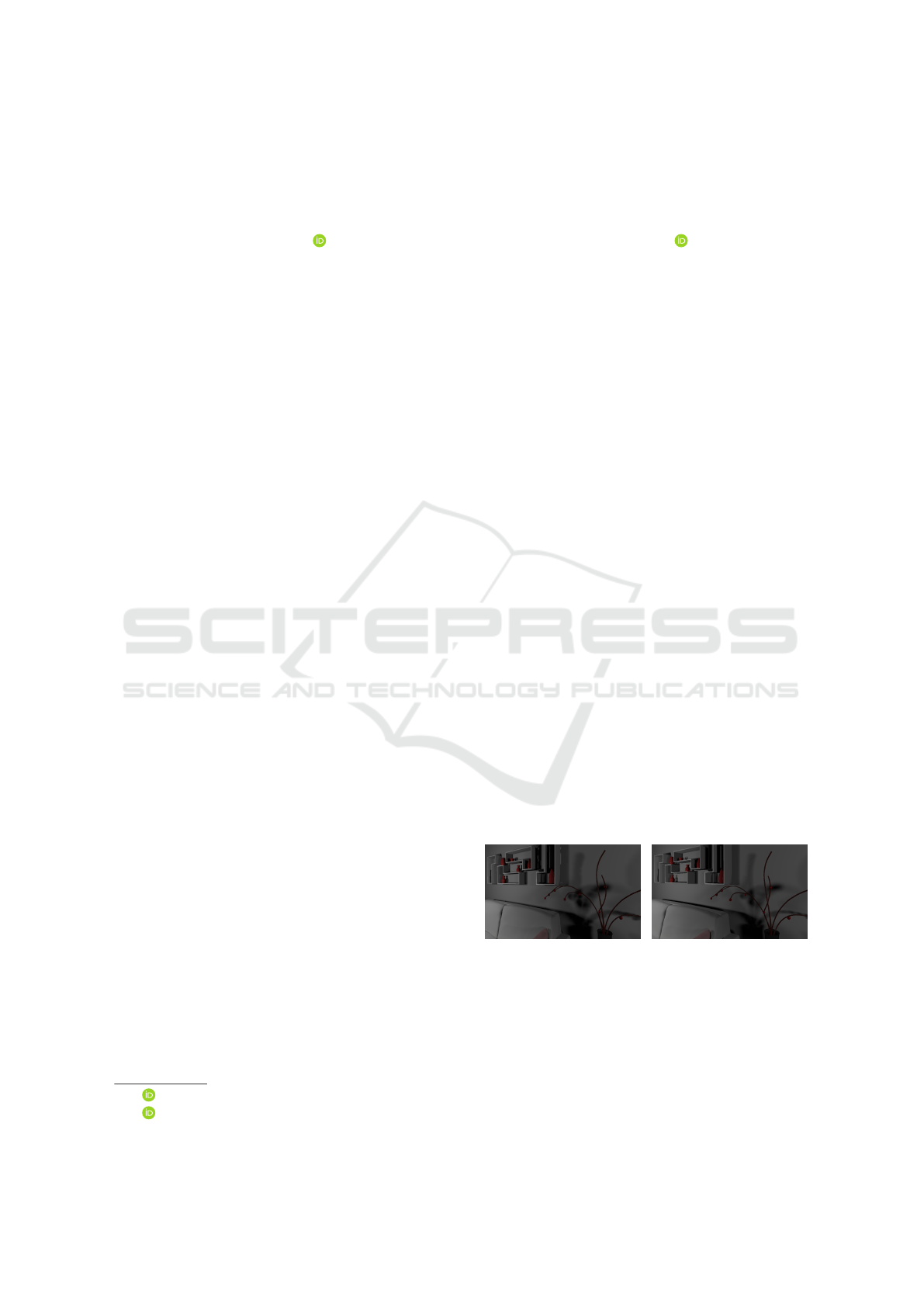
(a) Jump flooded SDF (b) Ray-traced SDF
Figure 1: Soft shadows from SDF raymarching.
2.1 Ray Tracing
The basic implementation of an SDF is a uniform grid
where the discrete points in the scalar field are stored
as a 3D texture (Wright, 2015). Uniform grids are
easy to implement and allow us to perform hardware
302
Tan, Y., Chua, N., Koh, C. and Bhojan, A.
RTSDF: Real-time Signed Distance Fields for Soft Shadow Approximation in Games.
DOI: 10.5220/0010996200003124
In Proceedings of the 17th International Joint Conference on Computer Vision, Imaging and Computer Graphics Theory and Applications (VISIGRAPP 2022) - Volume 1: GRAPP, pages
302-309
ISBN: 978-989-758-555-5; ISSN: 2184-4321
Copyright
c
2022 by SCITEPRESS – Science and Technology Publications, Lda. All rights reserved
interpolation of neighbouring points, making sam-
pling efficient. A brute force approach to generate
uniform SDF is ray sampling (Wright, 2015).
For each discrete point in the distance field, we
shoot rays in random directions to query the distance
to the closest mesh. To calculate the direction, we ran-
domly generate a point on the surface of a sphere with
a uniform distribution (Weisstein, 2019). The mini-
mum distance traced for each point is stored in the
red channel of a 400 × 200 × 400 3D texture. Rays
traced in future frames will overwrite the value if the
newer value is smaller. To determine the sign, we first
check if it is a front or back face hit via the dot prod-
uct of the ray direction and normal of the primitive
intersected. We then accumulate the number of front
and back face hits in the green and blue channels of
the texture. Finally, we set the sign to negative if the
majority of hits are back face hits (Wright, 2015).
2.2 Jump Flooding
The jump flooding algorithm (JFA) (Rong and Tan,
2006) which can be run on parallel on the GPU al-
lows us to generate an approximate SDF in real-time.
We first initialize a 3D SDF texture where each texel
represents a 3D point or a grid point. JFA gives us in-
formation about the closest seed at any point in space.
Setting every point on each triangle in the mesh as a
seed, we can obtain the closest distance to a surface
for our distance field. To determine if a grid point
contains a triangle efficiently, we voxelize the scene
with voxel resolution equal to our final distance field.
After voxelization, we simply check if a grid point
contains a model voxel to determine if it is a seed.
We now have a 3D texture containing grid points
that are either empty or are seeds. Without loss of
generality, we assume that the dimensions of the 3D
texture are equal (i.e. 3D cube) and that its length n
is a power of 2. For each grid point, we query a con-
stant number of neighbouring grid points a predefined
offset away. For each query, if the queried grid point
is a seed or contains seed information, we check if
that seed is closer to its currently stored seed and up-
date its seed information if so. We start with an offset
of length
n
2
and halve it for each subsequent iteration
until it reaches 1 for our final iteration.
With current GPUs that can write to 3D textures,
we adapt the 2D JFA algorithm (Rong and Tan, 2006)
for 3D space. During a single iteration, we run the
querying in parallel, allowing us to use the GPU to
accelerate the calculations. However, the algorithm
produces an unsigned distance field. To determine the
sign, we subtract a small β from the distance field,
causing surface points to be of negative value and ef-
fectively thickening the surface. The surfaces gener-
ated are also hollow as they contain positive values in
their interior. With jump flooding, we can generate
an approximate SDF in real-time for a decently large
resolution of 256
3
at 30ms and 128
3
at 2.34ms.
2.3 Ray Mask
We obtain a rough approximation of the SDF or
coarse SDF via jump flooding to locate regions in the
scene to apply ray tracing. In raymarching, regions
far from the surface act as a way to accelerate the pro-
cess but closer regions require a more accurate surface
representation. Hence, we can detect regions closer to
surfaces based on a distance d from the coarse SDF
and only ray trace in these regions at a higher resolu-
tion for better surface representation. Essentially, the
coarse SDF is a ray mask that determines which ar-
eas in the SDF should be ray-traced to generate a fine
SDF as shown in Figure 2. d can be used to trade-off
performance for accuracy where a larger d results in
more rays traced as texels further from surfaces would
be within d distance from a surface point.
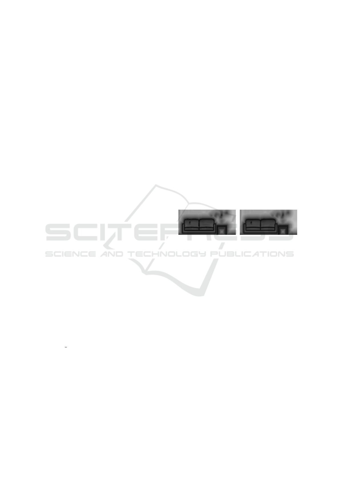
(a) Coarse SDF (b) Fine SDF
Figure 2: Slice of SDF.
Unlike adaptively sampled fields which increase
the resolution at regions with finer details, we limit
the number of levels of detail to two as generation
of hierarchical SDF is difficult to parallelize (Liu and
Kim, 2014). Additionally, real-time traversal of the
SDF may require multiple texture lookups to sample
until the leaf node despite saving space with a sparse
voxel texture (Aaltonen, 2018).
With the combination of the techniques, we turn
a blocky representation of the scene into a more re-
fined triangle mesh representation without ray tracing
every texel in the SDF as shown in Figure 3. Addi-
tionally, we can resolve issues identified in the jump
flooding of voxelization of thin surfaces. As seen in
Figure 4, while the coarse SDF gets a disconnected
representation of the plant, we fill in the holes through
refinement with the ray trace pass.
2.4 Raymarching
While SDFs are surface representations, they only
provide proximity information without a direction. To
perform ray casting on an SDF, we can find the inter-
section with raymarching. The SDF value shows the
RTSDF: Real-time Signed Distance Fields for Soft Shadow Approximation in Games
303
(a) Coarse SDF (b) Fine SDF
Figure 3: Precision.
(a) Coarse SDF (b) Fine SDF
Figure 4: Holes.
safest possible distance we can move along the ray
without missing any potential intersections. Hence,
given a ray origin and direction, we can query the
SDF at safe points along the ray and terminate if the
distance field returns a value less than or equal to 0,
signalling that we have reached a surface point.
This raymarching algorithm, also known as sphere
tracing (Hart, 1996), does not account for no inter-
section and could potentially iterate indefinitely in
practice. A simple solution would be to terminate if
the raymarched distance exceeds the bounds of the
queried scene. More commonly, we can set a max-
imum number of iterations to perform and return no
intersection if the limit is reached, ensuring consis-
tent execution time for interactive rendering. Ad-
ditionally, as the raymarch count approaches ∞, we
are marching closer to a surface but will never reach
it, potentially making the algorithm run indefinitely.
Hence, we could terminate the algorithm if the clos-
est distance to a surface is lower than some ε.
SDFs are used to calculate dynamic occlusion in
rendering like for area light shadow approximation as
in Wright (2015). Considering direct illumination of
the area light source alone, we can reform the ren-
dering equation as explained in Dutr
´
e et al. (2004).
Wright (2015) uses raymarching of SDFs to approxi-
mate the visibility term for the entire area light source.
With ray tracing, we can only get the intersection
point with the surface. However, we can also know
the closest it got to intersecting an object with ray-
marching. To get this information with ray tracing,
we need to shoot multiple rays within a cone which is
more accurate but too inefficient for real-time.
2.5 Correcting Artifacts
2.5.1 Ghosting
While the fine SDF generated is comparable to full
ray sampling, it uses temporal accumulation to con-
verge to the final distance field. Consequently, when
a moving object is introduced in the scene, its surface
ghosts as shown in Figure 5 because the area it leaves
is not invalidated as the closest distance.
Figure 5: Ghosting of circular-moving teapot.
(a) 128
3
coarse SDF input
(b) x = 1
(c) x = 5 (d) x = 10
Figure 6: Fine SDF result.
As such, each texel in the SDF must be recalcu-
lated every frame. However, to get stable results, the
number of rays x shot per frame must be substantially
high. Otherwise, it will result in noisy SDF as shown
in Figure 6 due to random sampling - in each frame,
there is a chance we might not hit the closest surface.
Conversely, the value of x is restricted by the com-
putational cost of ray tracing. As a compromise, we
spread our effective rays shot over multiple frames
with temporal accumulation of the SDF but apply a
GRAPP 2022 - 17th International Conference on Computer Graphics Theory and Applications
304
decay factor to the distance field in the previous frame
to minimize ghosting as shown in Equation 1.
f
t
=
(
min(α · f
t−1
+ (1 −α) · c
t
, r
t
), for c
t
≤ d
c
t
, for c
t
> d
(1)
Let f
t
, c
t
and r
t
be the fine SDF, coarse SDF and
the shortest distance generated from ray sampling re-
spectively at frame t. α refers to the decay factor for
the previous frame. Note that we eliminate any form
of ghosting for c
t
> d as we use c
t
, the jump flooded
SDF that is newly calculated every frame. To perform
jump flooding every frame, the coarse SDF is set to
128
3
while the fine SDF is at a resolution of 256
3
.
Our testing found an α of 0.95 and d of 0.1 provides
a good qualitative result which minimizes ghosting of
moving surfaces.
2.5.2 Banding
Banding artifacts come from the low resolution of the
SDF for real-time optimization. They appear along
the penumbra of shadows, causing alternating regions
of high and low occlusion as shown in Figure 7.
(a) Before triangu-
lation
(b) After triangula-
tion
(c) After triangula-
tion and max. step
size
Figure 7: Banding from low resolution SDF.
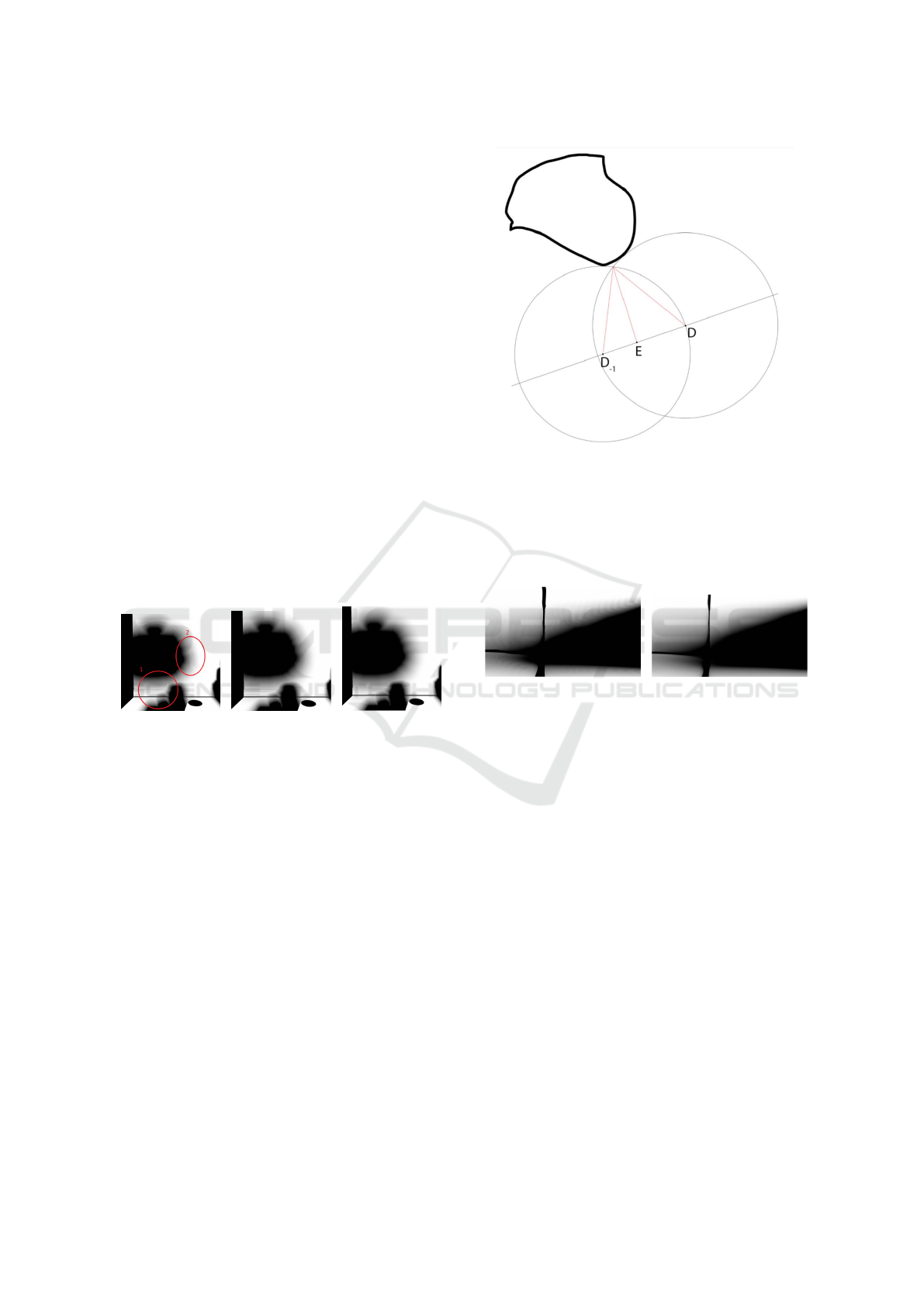
We reduce some of the banding by approximat-
ing the occlusion according to Aaltonen (2018). From
Figure 8, given two raymarch samples D and D
−1
, we
can triangulate to calculate an approximation of the
SDF at E which would have contributed to a higher
occlusion than both samples.
To ensure that neighbouring pixels have similar
raymarch samples, we also restrict the maximum step
size of our raymarching to 0.05 to remove the band-
ing. However, a consequence would be an increase
in texture samples (128 in this case) required to cal-
culate occlusion so we are looking into finding a bet-
ter compromise. Nonetheless, we achieve a smooth
penumbra for now, as expected of a soft shadow.
Lastly, due to the fixed step size, there is also an
obvious pattern when shadows are parallel to the light
direction. We remove this sampling artifact by jit-
tering the offset of the ray so that we move our ray
Figure 8: Approximation of occlusion with triangulation.
Source: Aaltonen (2018).
sample slightly along the light direction. We then ap-
ply a temporal anti-aliasing (TAA) (Karis, 2014) pass
to remove any noise in the final image for a smooth
gradient as shown in Figure 9.
(a) Before TAA (b) After TAA
Figure 9: Banding from fixed step size.
2.5.3 Holes
Holes in our SDFs are observable from the shadow of
objects with thin surfaces like in Figure 10 due to the
low resolution of the SDF. Increasing the resolution
to 500 × 500 × 500 only reduces the size of the holes
but does not eliminate them, and results in a poor ren-
dering performance of 70ms. Consequently, we add a
bias of 0.01 to our SDF to thicken surfaces. With this
change, we compromise the accuracy of the surface
representation for cleaner shadows.
Another artifact comes from the ε of our ray-
marching technique. ε must be minimally one voxel
size to avoid self-occlusion. However, the ray steps
through thin surfaces entirely due to the large ε aris-
ing from our low-resolution distance field, appear-
ing as holes in the shadow umbra as shown in Fig-
ure 11. A solution is to combine our soft shadow
technique with a classic hard shadow approach like
Cascaded Shadow Maps (CSM) (Engel, 2006) which
can achieve the shadow umbra.
RTSDF: Real-time Signed Distance Fields for Soft Shadow Approximation in Games
305
(a) Low resolution (b) High resolution
Figure 10: Holes in SDF.
Figure 11: Holes in umbra.
3 RESULTS
We test our RTSDF technique by generating ray-
marched soft shadows and comparing them with the
shadows produced by shadow mapping and ground
truth distributed ray tracing (Cook et al., 1984). Our
shadow map implementation makes use of the CSM
and Exponential Variance Shadow Maps (EVSM)
(Lauritzen and McCool, 2008) filtering sample pro-
vided by Falcor. We perform our evaluation on THE
MODERN LIVING ROOM (Wig42, 2014) with dy-
namic objects and TAA.
3.1 Performance
The measurements here are taken with the Falcor pro-
filing tool on an Intel Core i7-8700K CPU at 16GB
RAM with an NVIDIA GeForce RTX 2080 Ti GPU.
3.1.1 Comparison with Shadow Mapping
We evaluate the performance of RTSDF with one di-
rectional light as shown in Table 1. Without extensive
optimizations on the Falcor API and Direct3D level,
we are already achieving relatively interactive frame
rates and pass durations. In comparison, shadow map-
ping has a frame rate of 241 fps, but it is expected that
our method is slower because of our additional SDF
generation and raymarching processes. We are also
using additional abstractions and wrappers provided
by Wyman (2018) for ease of implementation.
Table 1: RTSDF pass durations (ms) and frame rate.
Passes Processor Duration
CPU 0.29
G-Buffer
GPU 1.05
CPU 0.63
Voxelization (V)
GPU 0.93
CPU 0.06
Jump Flood (JF)
GPU 2.09
CPU 1.05
Ray Trace (RT)
GPU 4.60
CPU 0.11
Deferred Lighting (DL)
GPU 1.28
CPU 7.42
Others
GPU 0.27
CPU 9.56
Total Duration
GPU 10.22
Frame Rate 97
3.1.2 SDF Resolution
We compare the increasing size of our SDF and
record the GPU timings for the SDF generation passes
and final deferred lighting computation on three lights
at different resolutions specified in Table 2.
Table 2: Resolution for different SDF sizes.
Resolution Coarse SDF Fine SDF
Small (S) 64
3
128
3
Medium (M) 128
3
256
3
Large (L) 256
3
512
3
As seen in Table 3, the duration of jump flood-
ing becomes much higher with increasing SDF reso-
lution, as there are more dispatch calls when execut-
ing the compute shader as well as reduced GPU cache
locality when reading and writing to a much larger
3D texture. Jump flooding for 256
3
coarse SDF costs
21.89ms which results in a frame rate of lower than
60 frames per second. Consequently, we note that
with current optimizations applied to jump flooding,
we are limited to 128
3
resolution. Nonetheless, with
a lower fine SDF resolution of 256
3
, we can afford to
shoot more rays per texel which improves the stability
of the distance field generated.
However, at 64
3
, the jump flooding is unable to
capture some surfaces of thin objects as seen in Fig-
GRAPP 2022 - 17th International Conference on Computer Graphics Theory and Applications
306
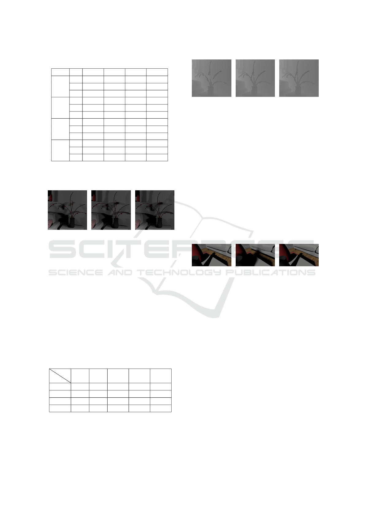
Table 3: GPU timings of passes (ms).
Size x 0 1 5 10
S 0.49 0.49 0.49 0.49
M 0.49 0.49 0.49 0.49
V
L 1.12 1.12 1.12 1.12
S 0.28 0.28 0.28 0.28
M 2.37 2.37 2.37 2.37
JF
L 21.89 21.89 21.89 21.89
S 0.14 0.16 0.71 1.41
M 0.55 1.41 4.51 8.36
RT
L 3.98 9.12 26.56 48.32
S 3.17 3.17 3.17 3.17
M 3.17 3.17 3.17 3.17
DL
L 7.32 7.32 7.32 7.32
ure 12 where the plant’s shadow is disjointed and in-
complete. Increasing the ray count gives little notice-
able improvement as the ray mask is too small.
(a) S (b) M (c) L
Figure 12: Thin object shadows.
3.1.3 Ray Mask Size
We measure the effect of distance d which determines
the size of the ray mask in Table 4. Here, d = ∞ cor-
responds to the case where every texel in the fine SDF
is ray-traced. As shown in Figure 13, there are notice-
able holes in the SDF for d = 0.05 as the low resolu-
tion of the coarse SDF makes it difficult to voxelize
thin surfaces. Increasing d to 0.1 fills up the missing
holes as we use a more aggressive ray mask which can
detect the thin surfaces. However, there is less quali-
tative difference from d = 0.1 to d = 0.5. Weighing it
against the decrease in performance, it appears that d
= 0.1 is most suitable for the shot.
Table 4: Size M SDF GPU timings (ms).
x
d
0.01 0.05 0.1 0.5 ∞
1 0.8 1.28 1.63 3.12 4.08
5 1.43 3.17 4.82 11.71 16.15
10 2.18 5.41 8.36 22.25 30.69
15 3.17 7.7 12.42 32.7 46.0
(a) d = 0.05 (b) d = 0.1 (c) d = 0.5
Figure 13: Thin surfaces.
3.2 Graphics Quality
We compare the smoothness of the soft shadow
penumbra generated with our approach against
shadow mapping as well as the ground truth as shown
in Figure 14 with one directional light. RTSDF gen-
erates a plausible penumbra while the penumbra from
shadow mapping is hardly visible. For shadow map-
ping, a 15px × 15px kernel was used to generate soft
shadows by blurring with EVSM filtering. It could
be the case that the shadow map resolution is too low
in the foreground for better quality penumbra. We
manage to recreate the details of the penumbra more
clearly such that it is closer to the distributed ray trac-
ing reference. Our penumbra appears to be larger than
the ground truth as a result of adding the small bias in
Section 2.5.3 to prevent holes in thin surfaces.
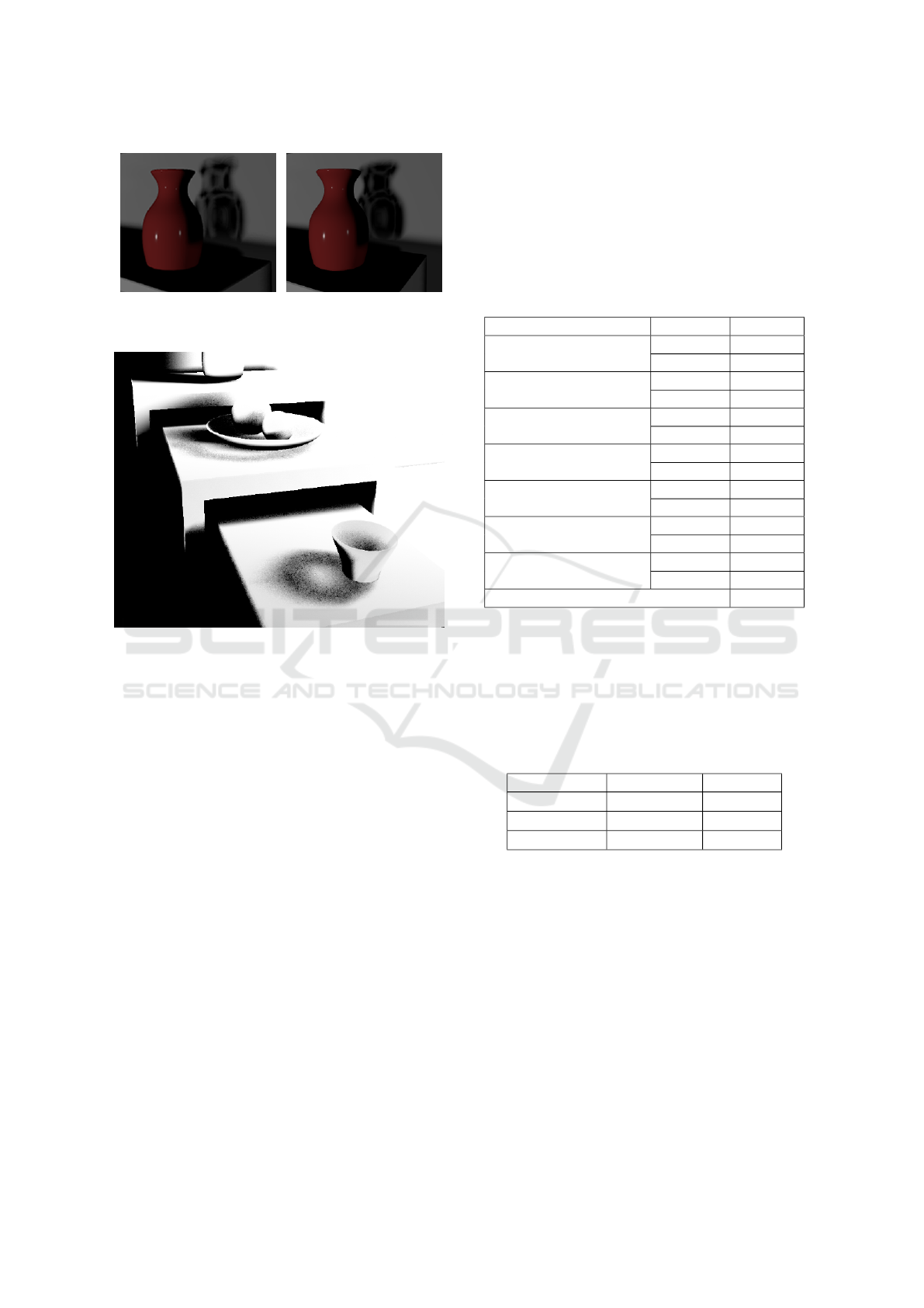
(a) Shadow Map (b) RTSDF (c) Distributed RT
Figure 14: Penumbra.
3.3 Limitations
Due to a small amount of ghosting of the SDF, our
rays shot towards the light source may intersect with
the ghosted surface representation of the object. This
results in incorrectly occluded areas such as the top of
the teapot in Figure 15. For static regions, this artifact
would not be present.
Though not a focus of the paper, a key thing to
note is also the accuracy of the shadows. Our soft
shadow algorithm widens the penumbra and does not
accurately calculate umbra as shown in Figure 16. On
the left, for the ground truth, we shoot multiple vis-
ibility rays towards the area light source and hence
have an occlusion factor of more than 0. However,
for the SDF raymarching estimation, we raymarch a
single ray towards the centre of the light source and
record an occlusion factor of 0. Consequently, this
technique is referred to as penumbra widening shad-
ows by Aaltonen (2018).
RTSDF: Real-time Signed Distance Fields for Soft Shadow Approximation in Games
307
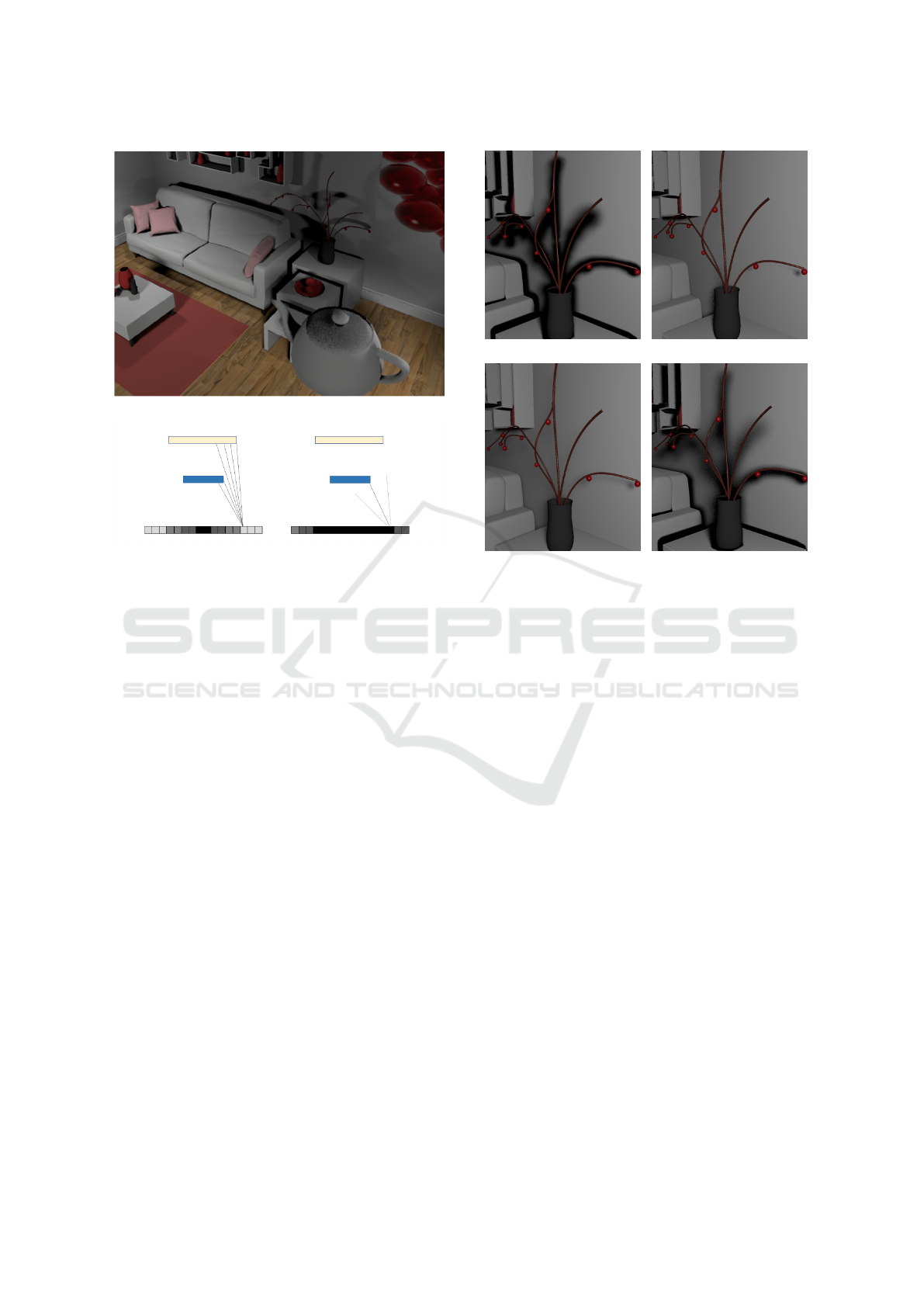
Figure 15: Self intersection of moving teapot.
Figure 16: Reference (left) vs penumbra estimation (right).
This becomes noticeable as we increase the ra-
dius of our area light source, and accompanied by
the increased thickness of the surface representa-
tion causes our shadows to substantially thicken and
darken. More research could be done to investigate
potential ways to calculate the shadow umbra given
an SDF to achieve less noisy results than a ray trace
counterpart. For example, as shown in Figure 17, we
could perform random sampling towards the light and
weight the occlusion factor based on the distance to
the closest object along the ray towards the light.
3.4 Future Work
3.4.1 SDF
Currently, the setup is fine-tuned for a small simple
scene. However, it gets more complex when account-
ing for larger scenes. Having a single SDF for the en-
tire scene is not feasible due to the memory and com-
putation requirements to get a good resolution per m
3
of the scene. A potential strategy would be to have a
clip map explained by Panteleev (2014), with multiple
resolutions based on the camera’s position and view
direction. In regions outside of the camera’s view
frustum, a lower resolution SDF can be calculated
which would reduce the cost of rendering. Further-
more, these regions could potentially use only jump
flooding instead of adding ray tracing.
As of the date of submission, the acceleration
(a) RTSDF (b) Ray Trace (1 per frame)
(c) Distributed Ray Trace (d) SDF-Simulated Umbra
Figure 17: Umbra.
structures generated by the GPU drivers which sup-
port the DirectX Raytracing API are not accessible in
code. They are bounding volume hierarchies that are
used for ray tracing and the API exposed only allows
for ray tracing queries. As noted by Quilez (2019),
proximity information can be queried from the accel-
eration structures and potentially be used for render-
ing effects. These structures could also help aid better
reconstruction of the SDF.
3.4.2 Soft Shadows
Currently, we apply TAA to reduce noise in the im-
age as shown in Figure 18. However, noise is not
eliminated. We could adopt ideas from existing tech-
niques such as spatiotemporal variance-guided filter-
ing (Schied et al., 2017) which uses screen space blurs
and temporal accumulation to remove noise from path
tracing samples. With more intelligent filtering of
the final result, we could potentially get away with
a larger raymarch step introduced to remove banding
artifacts and improve performance.
Raymarching is an expensive operation given the
required number of samples per pixel. We could also
optimize this by combining our soft shadows with a
shadow map pass where we decide to raymarch only
if not in shadow.
While not explored, we note that since we have
an SDF approximation of the scene, there is the po-
GRAPP 2022 - 17th International Conference on Computer Graphics Theory and Applications
308

(a) Before TAA (b) After TAA
Figure 18: Noise.
tential of representing translucent surfaces to gener-
ate translucent soft shadows. The main initial dif-
ficulty would be identifying the surface intersected
when raymarching a distance field. We could poten-
tially store surface information in the distance field
and perform optimization by using lookup tables.
4 CONCLUSION
We developed a novel technique that combines jump
flooding and ray tracing to generate SDFs in real-time
with plausible results for soft shadowing and exposed
values that trade-off between performance and qual-
ity of the SDF generated which would be useful when
targeting hardware of different specifications. Our ap-
proach can handle scenes with dynamic objects and
produce penumbra that is smoother than shadow map-
ping but cleaner than distributed ray tracing.
ACKNOWLEDGEMENTS
We thank Wyman (2018) for the Falcor scene file of
THE MODERN LIVING ROOM (CC BY). This work
is supported by the Singapore Ministry of Educa-
tion Academic Research grant T1 251RES1812, “Dy-
namic Hybrid Real-time Rendering with Hardware
Accelerated Ray-tracing and Rasterization for Inter-
active Applications”.
REFERENCES
Aaltonen, S. (2018). Advanced graphics techniques tuto-
rial: Gpu-based clay simulation and ray-tracing tech
in ’claybook’.
Benty, N., Yao, K.-H., Clarberg, P., Chen, L., Kallweit,
S., Foley, T., Oakes, M., Lavelle, C., and Wyman, C.
(2020). The Falcor rendering framework.
Cook, R. L., Porter, T., and Carpenter, L. (1984). Dis-
tributed ray tracing. SIGGRAPH Comput. Graph.,
18(3):137–145.
Dutr
´
e, P., Jensen, H. W., Arvo, J., Bala, K., Bekaert, P.,
Marschner, S., and Pharr, M. (2004). State of the art in
monte carlo global illumination. In ACM SIGGRAPH
2004 Course Notes, SIGGRAPH ’04, page 5–es, New
York, NY, USA. Association for Computing Machin-
ery.
Engel, W. (2006). Cascaded shadow maps. pages 197–206.
Hart, J. (1996). Sphere tracing: A geometric method for the
antialiased ray tracing of implicit surfaces. The Visual
Computer, 12:527–545.
Karis, B. (2014). High quality temporal supersampling.
Lauritzen, A. and McCool, M. (2008). Layered variance
shadow maps. In Proceedings of Graphics Interface
2008, GI ’08, page 139–146, CAN. Canadian Infor-
mation Processing Society.
Liu, F. and Kim, Y. J. (2014). Exact and adaptive signed
distance fields computation for rigid and deformable
models on gpus. IEEE Transactions on Visualization
and Computer Graphics, 20(5):714–725.
Panteleev, A. (2014). Practical real-time voxel-based global
illumination for current gpus. GTC 2014.
Quilez, I. (2019). Sdf bounding volumes - 2019.
Rong, G. and Tan, T.-S. (2006). Jump flooding in gpu with
applications to voronoi diagram and distance trans-
form. In Proceedings of the 2006 Symposium on
Interactive 3D Graphics and Games, I3D ’06, page
109–116, New York, NY, USA. Association for Com-
puting Machinery.
Schied, C., Kaplanyan, A., Wyman, C., Patney, A., Chai-
tanya, C. R. A., Burgess, J., Liu, S., Dachsbacher,
C., Lefohn, A., and Salvi, M. (2017). Spatiotempo-
ral variance-guided filtering: Real-time reconstruction
for path-traced global illumination. In Proceedings
of High Performance Graphics, HPG ’17, New York,
NY, USA. Association for Computing Machinery.
Tan, Y. W., Chua, N., Koh, C., and Bhojan, A. (2020).
RTSDF: Generating Signed Distance Fields in Real
Time for Soft Shadow Rendering. In Lee, S.-h., Zoll-
mann, S., Okabe, M., and Wuensche, B., editors, Pa-
cific Graphics Short Papers, Posters, and Work-in-
Progress Papers. The Eurographics Association.
Weisstein, E. W. (2019). Sphere point picking.
Wig42 (2014). The modern living room.
Wright, D. (2015). Advances in real-time rendering in
games: Part ii: Dynamic occlusion with signed dis-
tance fields.
Wyman, C. (2018). Introduction to directx raytracing. In
ACM SIGGRAPH 2018 Courses, SIGGRAPH ’18.
RTSDF: Real-time Signed Distance Fields for Soft Shadow Approximation in Games
309
