A Light Source Calibration Technique for Multi-camera Inspection

Devices

Mara Pistellato

, Mauro Noris, Andrea Albarelli

and Filippo Bergamasco

DAIS, Universit

a Ca’Foscari Venezia, 155, via Torino, Venezia, Italy

Keywords:

Light Source Calibration, Multi-camera, Inspection Devices.

Abstract:

Industrial manufacturing processes often involve a visual control system to detect possible product defects

during production. Such inspection devices usually include one or more cameras and several light sources

designed to highlight surface imperfections under different illumination conditions (e.g. bumps, scratches,

holes). In such scenarios, a preliminary calibration procedure of each component is a mandatory step to

recover the system’s geometrical conﬁguration and thus ensure a good process accuracy. In this paper we

propose a procedure to estimate the position of each light source with respect to a camera network using an

inexpensive Lambertian spherical target. For each light source, the target is acquired at different positions

from different cameras, and an initial guess of the corresponding light vector is recovered from the analysis

of the collected intensity isocurves. Then, an energy minimization process based on the Lambertian shading

model reﬁnes the result for a precise 3D localization. We tested our approach in an industrial setup, performing

extensive experiments on synthetic and real-world data to demonstrate the accuracy of the proposed approach.

1 INTRODUCTION

Light source estimation is a crucial task in several

computer vision tasks, especially while performing

visual inspection activities. Indeed, such informa-

tion can be exploited to generate synthetic images

with different illuminations in order to detect possi-

ble defects. Illuminant estimation is also needed in

shape-from-shading techniques, where a scene is re-

constructed observing its features in images acquired

with a changing illumination (Zheng et al., 2002;

Samaras and Metaxas, 2003; Wang et al., 2020).

Light estimation is also beneﬁcial in many other ﬁelds

such as cultural heritage (Fassold et al., 2004; Pistel-

lato et al., 2020) or augmented reality, where new ob-

jects can be rendered onto the acquired image simu-

lating realistic shadings (Sato et al., 1999a; Wang and

Samaras, 2003).

The literature counts a number of heterogeneous

approaches for light source estimation, depending on

the target application and its requirements. In some

cases the light source is calibrated in conjunction to

other specialised tasks as dense SLAM (Simultane-

ous Localization And Mapping) (Whelan et al., 2016)

https://orcid.org/0000-0001-6273-290X

https://orcid.org/0000-0002-3659-5099

https://orcid.org/0000-0001-6668-1556

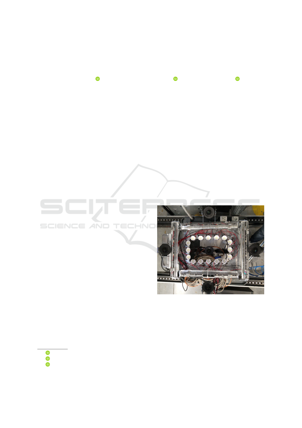
Figure 1: Picture of our inspection device. It includes ﬁve

cameras and sixteen punctual lights uniformly distributed in

a rectangle around the central camera.

or camera calibration (Cao and Shah, 2005). Some

tasks require the localisation of directional sources,

as in (Pentland, 1982), where the direction of lights at

inﬁnity are estimated (e.g. daylight). Several shape-

from-shading approaches adopt this kind of model,

since the light direction is sufﬁcient for the recon-

struction task (Zheng et al., 2002; Brooks and Horn,

1985; Zhang et al., 1999). In (Zhou and Kamb-

hamettu, 2002) multiple light sources are estimated

488

Pistellato, M., Noris, M., Albarelli, A. and Bergamasco, F.

A Light Source Calibration Technique for Multi-camera Inspection Devices.

DOI: 10.5220/0010995900003122

In Proceedings of the 11th International Conference on Pattern Recognition Applications and Methods (ICPRAM 2022), pages 488-494

ISBN: 978-989-758-549-4; ISSN: 2184-4313

using a stereo camera setup and a sphere: the method

involves an algorithm to separate Lambertian from

specular intensity and devise direction and intensity

of the light sources. In (Li et al., 2003) the authors

propose an uniﬁed framework integrating shading,

shadows and specular cues to devise the light direc-

tion. In some scenarios the directional assumption is

not valid: for instance if we have artiﬁcial illumina-

tion in a small room. These situations require the light

to be modelled as a point source, so its exact position

in 3D space is to be recovered. Most of these tech-

niques exploit some priors on the scene geometry, as

in (Debevec, 2008; Sato et al., 1999a). This is limiting

in many scenarios, since the knowledge of the scene is

often not available or requires a signiﬁcant computa-

tional effort. Moreover, several methods estimate the

illumination as a radiance map, losing the information

about light location (Sato et al., 1999b; Kim et al.,

2001). In (Powell et al., 2001; Powell et al., 2000)

the authors propose to use three spheres with known

relative positions as a target for light position estima-

tion, while in (Takai et al., 2009) both point and di-

rectional light sources are estimated employing a pair

of spheres and computing the intensity difference of

two regions of such objects. The work in (Langer and

Zucker, 1997) tries to unify different kinds of light

sources, introducing a 4-dimensional hypercube rep-

resentation where different types of lights can be em-

bedded, while the method proposed in (Jiddi et al.,

2016) exploits and RGB-D sensor to estimate the lo-

cation of light sources using only the specular re-

ﬂections observed on the scene. Recently, some au-

thors proposed learning-based methods to perform the

same task. In (K

an and Kafumann, 2019) the authors

propose a CNN (Convolutional Neural Network) to

devise lighting information exploiting a dataset of im-

ages with known light sources. Other examples are

(Gardner et al., 2017; Elizondo et al., 2017).

In our approach we propose a light calibration pro-

cedure for a multi-camera network using a Lamber-

tian spherical object with uniform albedo as light cal-

ibration target. First, the sphere is detected in each

camera in order to compute its accurate 3D position,

then we carry out a coarse initialisation exploiting the

intensity isocurves extracted from the sphere’s sur-

face. After that, we reﬁne the light position formu-

lating an optimisation over the observed intensity val-

ues based on the Lambertian shading model. Our ap-

proach is particularly suitable in scenarios where the

device setup is mutable and thus an inexpensive (in

terms of both time and convenience) light calibration

approach is required.

2 LIGHT CALIBRATION

TECHNIQUE

Our surface inspection device is shown in Figure 1.

It is composed by a network of ﬁve 12-Megapixels,

grayscale cameras pointing towards the same direc-

tion and mounted on a rigid structure. The illumina-

tion system includes 16 punctual led lights, uniformly

distributed in a rectangle around the central camera,

approximately at the same height of lateral cameras.

In order to correctly simulate scene illuminations and

identify surface anomalies, we are interested in esti-

mating the light locations with respect to the camera

network. However, the cameras are mounted around

and below the main frame and are subject to modi-

ﬁcations, thus it is not possible to accurately locate

the lights according to the original device blueprint.

For this reason, we assume to know only the network

imaging model and we aim to infer the light sources

positions by observing an object with a characteristic

shading model.

Our calibration procedure works for each light

source independently. A matte white sphere is sus-

pended in front of the cameras at N different posi-

tions, keeping only the desired light source turned on.

Note that the sphere is characterized by a constant

albedo to avoid camera integration problems (Pistel-

lato et al., 2018). The device captures the illuminated

sphere, resulting in a set of N images I

...I

for each

camera, with i = 1,..., T . The sphere reﬂectance

model is then taken into account to infer the light po-

sition from the observed images, as described in the

following sections.

2.1 Light Position Optimization

The target sphere S

projects to a circle

in each ac-

quired image I

. A RANSAC-based detector is used

to locate the circle in the image, then a least-square ﬁt-

ting approach is applied to accurately locate the centre

with sub-pixel precision.

The rays originating from each camera’s optical

center and passing through the circle centers are then

triangulated using (Pistellato et al., 2016; Pistellato

et al., 2015) to obtain the 3D position of the sphere

)

with respect to the camera network ref-

erence frame (corresponding to the central camera in

our case). Note that, since both intrinsic and extrinsic

parameters are calibrated, the radius of S

is not im-

portant to recover its position, that can be estimated a-

The projection is actually a conic, but we believe that

a circle is a fair approximation for this task, excluding ex-

treme cases when the sphere is imaged at camera borders.

A Light Source Calibration Technique for Multi-camera Inspection Devices

489

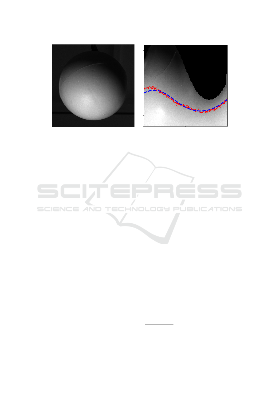
Figure 2: Acquired intensity image (left) and sphere surface remapped in spherical coordinates (right). The isocurve P

corresponding to the intensity level 160 is shown in red. The blue dashed line is the curve corresponding to the winning bin

in the accumulator.

posteriori comparing the circle radius with the sphere

depth.

We assume that the reﬂectance of the matte white

sphere used as target can be well approximated by the

Lambertian model (Koppal, 2014), plus some (non-

directional) ambient light scattered from the rest of

the scene. We deﬁne the light source as a 3D point L ∈

; then the intensity of the light I

(p) reﬂected from

the point p, lying onto the sphere surface, is modelled

as:

(p) = N(p)

L(p)I

+ a (1)

where N(p) ∈ S

is the surface normal at p, L ∈ S

is the (unitary-norm) light vector originating from p

and pointing towards the light (ie: L(p) =

L−p

kL−pk

), I

is the light (scalar) intensity and a is the ambient con-

tribution.

When the sphere is imaged by a camera, each

point p ∈ S is projected to a pixel location p

. If p

given, the corresponding sphere point p is obtained by

intersecting the ray originating from p

with S. There-

fore, to recover L we can iterate through all the pixels

belonging to the circle on the image and compare their

intensities with the expected intensities given by (1).

However, the image of each camera may differ from

that model for several reasons:

• The Camera Response Function (CRF) is in gen-

eral non-linear;

• Each camera might have a different gain, exposure

and iris setting;

• The image intensity is quantized to 8 bits and

clipped to a range between 0 and 255.

To partially account these problems, we explicitly

model the intensity clipping due to the quantized cam-

era values. Moreover, we let the “apparent” light in-

tensity I

and the ambient contribution a to be image

dependent, deﬁning I

and a

as light intensity and

ambient contribution for n

sphere position and i

camera.

We formulate light calibration as the following non-

linear minimization problem:

min

∑

n=1

∑

i=1

∑





N(p

)

L(p

+ a



− (2)

−I

)



+ αkL

−

where β = (L,I

,. .. ,I

,. .. ,a

) is the vector of

unknowns to be estimated, containing the 3 coordi-

nates of L, the light intensity and ambient contribution

for each separate image.

Since the lights mounting frame is at a ﬁxed ele-

vation with respect to the central camera, the regular-

ization term kL

−

k forces the light z-coordinate to

remain between a reasonable elevation

. Note that

and L

can instead freely move. Finally, C models

the camera intensity clipping, and is simply deﬁned

as C(x) = max(min(x,255),0).

In our implementation, Equation 3 is numeri-

cally solved with the BFGS algorithm (Nocedal and

Wright, 2006) using the gradient that is symbolically

evaluated by the TensorFlow library. Being a gradi-

ent descent approach, a reasonable starting condition

for β must be provided to let the optimization process

converge.

We empirically observed that a value of α = 10

−4

enough to ensure the convergence of the optimization while

not constraining too much the light elevation.

ICPRAM 2022 - 11th International Conference on Pattern Recognition Applications and Methods

490

5 10 15 20 25

Samples

MAE (mm)

Lights#5-#13distanceMAE

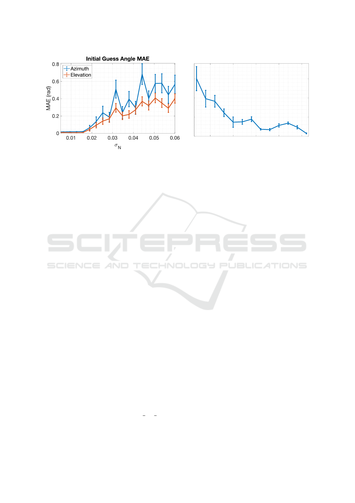
Figure 3: Left: initial estimation errors for the light vector increasing the value of additive noise σ

. Right: real-world

experiment showing MAE of the distance between two lights varying the number of samples.

2.2 Guessing the Initial Conﬁguration

Due to the interplay between the dot product N

L and

the image-dependent light intensity I

, an initial value

of β can be difﬁcult to guess. However, if the sphere

radius is small compared to the light distance, the vec-

tor L − p is well approximated by L − (c

). In

other words, there is no appreciable difference be-

tween a light L and a light placed inﬁnitely far away

from S in the direction L − (c

). Therefore,

the pixel-dependent L(p) can be substituted with the

image-dependent normalized light direction L

∈ S

Since N and L

are both unit vectors, it is con-

venient to represent them in spherical coordinates as

N(s) = (φ

,θ

)

and L

= (φ

,θ

)

, where s is a

point lying on the sphere, φ is the azimuth angle with

respect to the x-axis and θ is the elevation angle with

respect to the y-axis.

From the circle C

we choose the isocurve of

points P

= {s

.. .s

} corresponding to a certain ar-

bitrarily intensity. Note that the intensity value is not

important, as long as the number of extracted points

m is reasonably large. Since the intensity I

(p) is con-

stant for the points in P

, Equation 1 can be rewritten

as k = N(s)

or, in spherical coordinates:

k = sin(θ

)

sin(θ

)+cos(θ

)

cos(θ

)cos(φ

−φ

(3)

Equation 3 deﬁnes the locus of points s

on the sphere

(corresponding to the image points s

) for which the

dot product between the surface normal and the light

vector is constant.

The advantage of this formulation is that the range

of values for θ, φ and k is limited to a restricted inter-

val. Speciﬁcally, φ ∈ {−π .. .π}, θ ∈ {−

.. .

} and

k ∈ {−1 .. .1} (dot product of unit vectors). For this

reason, we can efﬁciently create a 3-dimensional ac-

cumulator for (θ

, φ

, k) to accumulate votes from

all the isocurve points.

The procedure works as follows: for each point

we enumerate all the triplets (θ

, φ

, k) for

which Equation 3 holds, and the accumulator bin cor-

responding to that parameter combination is incre-

mented by one. Since L

and −L

deﬁne the same

light ray in space, we restrict the enumeration to the

triplets with a positive value of k (i.e. the angle be-

tween N and L

is less than π/2). When the accu-

mulator is ﬁlled, the location of the maximum gives a

good approximation of the light direction vector L

and the parameter k. Figure 2 shows an example

of acquired intensity image (left) and corresponding

remapping in spherical coordinates (right), where an

isocurve is highlighted together with the winning ac-

cumulator bin.

The described procedure is repeated for all the N

images to obtain a set of rays in space passing trough

)

and with direction L

. Finally, the 3D

point closest to all such rays is used as the initial light

location for the optimisation (3).

3 EXPERIMENTAL EVALUATION

In order to assess the quality and stability of the pro-

posed light calibration method, we performed both

synthetic and real-world experiments presented in this

section.

Since ground truth data for exact position of a light

source is not always available nor accurate, we ﬁrst

tested the stability of the initialisation step exploiting

synthetic data.

We generated a random light vector and rendered part

of the observed sphere surface according to each cam-

era viewpoint. The intensity values were perturbed

A Light Source Calibration Technique for Multi-camera Inspection Devices

491

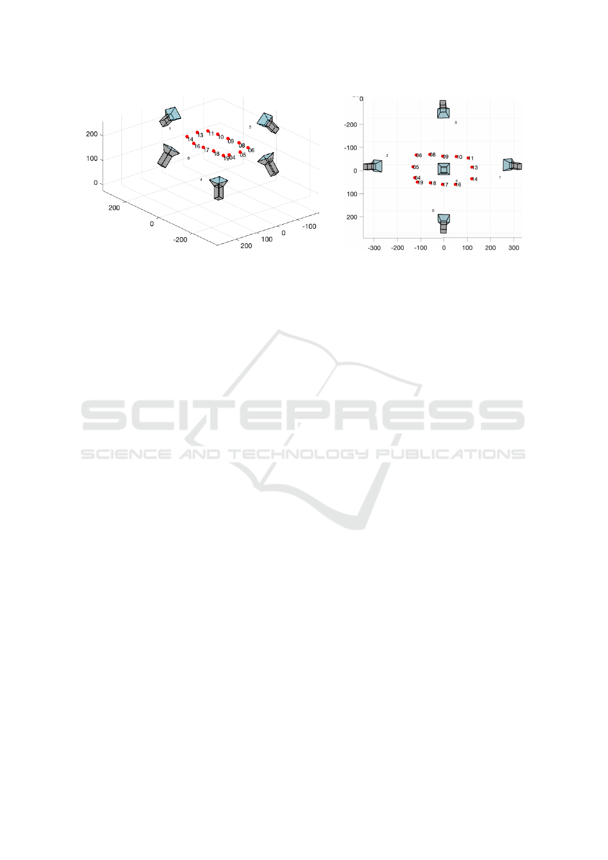
Figure 4: Qualitative results for the ﬁnal calibrated system with 5 cameras and 14 lights.

with a zero-mean Gaussian noise of standard devia-

tion σ

, then such data is used to extract the isocurves

and compute the light direction.

We used an accumulator of size 50 × 50 × 100 to col-

lect the votes from each isocurve point. The curves in

Figure 3 (left) show the mean absolute errors of the

initial guess with respect to the ground truth vector in

terms of azimuth and elevation angles. We increased

the value of σ

from 0.005 up to 0.06 and repeated

each test 100 times using random light directions and

sphere areas. The error bars denote the standard error

for each σ

In general, error values are low for σ

smaller than

0.02, then they rise up to 0.4 radians for very high

noise levels. This conﬁrms the stability and accuracy

offered by the proposed initialisation.

3.1 Real-world Experiments

We validated the proposed method using real-word

data acquired with our setup shown in Figure 1. The

whole camera network has been previously calibrated

for both the intrinsics and extrinsics parameters.

We used a target sphere with a radius of 45mm

and acquired the pictures by triggering the cameras

at the same time for each different light separately.

The object was hanged above the device, spanning

the intersection of cameras frustums. We then moved

the sphere in 7 different locations, obtaining 16 (one

for each light) sets of ﬁve images for each different

sphere location.

Note that since the sphere slightly moved during

acquisitions, we triangulated its position for each light

independently using the whole camera network. This

was done by ﬁrst detecting the circular contour in the

images, and then triangulating the 3D position of the

sphere as already described.

According to the previous discussion, accurate

light positions within the cameras reference frame can

not be known a priori. For this reason we tested

the stability of our method in the real-world sce-

nario analysing the relative distance for a speciﬁc pair

of lights for which the value is known by construc-

tion. We chose two speciﬁc lights (number 5 and

13, displayed in Figure 4) located at opposite sides of

the rectangular structure and computed their positions

with our technique.

In Figure 3 (right) we show the mean absolute er-

ror of the computed distances with respect to the real

distance between the selected lights.

In order to test the impact of the number of sam-

ples on the estimation precision, we varied the num-

ber of images used for the calibration procedure (from

2 to 26, shown in the x-axis) and repeated the exper-

iment 20 times, randomly selecting the images from

the whole dataset. The plot exhibits a clear decreas-

ing trend as the number of samples increases, starting

from an average error of 15mm in the case of two im-

ages, reaching a millimetric precision with more than

15 samples. Also the standard error decreases with

the number of samples, denoting a good algorithm

stability.

Finally, in Figure 3 (second row) we show qualita-

tive results displaying the ﬁnal conﬁguration obtained

after the optimisation of all the lights (note that the

displayed output does not correspond to the original

light conﬁguration). Lights are plotted as red dots

with their corresponding IDs, together with the ﬁve

cameras.

The lights are almost coplanar and follow the rectan-

gular structure mounted on the device around the cen-

tral camera. Small deviations from the frame are due

to local adjustments that bring the lights to be slightly

misaligned with respect to the structure.

ICPRAM 2022 - 11th International Conference on Pattern Recognition Applications and Methods

492

4 CONCLUSIONS

In this paper we presented a light estimation tech-

nique particularly designed for a multi-camera in-

spection system in industrial environments.

Our approach exploits the observed intensities in the

spherical coordinates to easily compute an initial

coarse initialisation with a 3D accumulator, then the

optimal light position is computed via an optimisation

procedure.

Both synthetic and real-world experiments demon-

strated the stability and the precision in the localisa-

tion of multiple light sources.

REFERENCES

Brooks, M. J. and Horn, B. K. (1985). Shape and source

from shading.

Cao, X. and Shah, M. (2005). Camera calibration and light

source estimation from images with shadows. In 2005

IEEE Computer Society Conference on Computer Vi-

sion and Pattern Recognition (CVPR’05), volume 2,

pages 918–923. IEEE.

Debevec, P. (2008). Rendering synthetic objects into real

scenes: Bridging traditional and image-based graphics

with global illumination and high dynamic range pho-

tography. In ACM SIGGRAPH 2008 classes, pages

1–10.

Elizondo, D. A., Zhou, S.-M., and Chrysostomou, C.

(2017). Light source detection for digital images in

noisy scenes: a neural network approach. Neural

Computing and Applications, 28(5):899–909.

Fassold, H., Danzl, R., Schindler, K., and Bischof, H.

(2004). Reconstruction of archaeological ﬁnds using

shape from stereo and shape from shading. In Proc.

9th Computer Vision Winter Workshop, Piran, Slove-

nia, pages 21–30.

Gardner, M.-A., Sunkavalli, K., Yumer, E., Shen, X., Gam-

baretto, E., Gagn

e, C., and Lalonde, J.-F. (2017).

Learning to predict indoor illumination from a single

image. arXiv preprint arXiv:1704.00090.

Jiddi, S., Robert, P., and Marchand, E. (2016). Reﬂectance

and illumination estimation for realistic augmenta-

tions of real scenes. In 2016 IEEE International Sym-

posium on Mixed and Augmented Reality (ISMAR-

Adjunct), pages 244–249. IEEE.

an, P. and Kafumann, H. (2019). Deeplight: light source

estimation for augmented reality using deep learning.

The Visual Computer, 35(6):873–883.

Kim, T., Seo, Y.-D., and Hong, K.-S. (2001). Improving ar

using shadows arising from natural illumination dis-

tribution in video sequences. In Proceedings Eighth

IEEE International Conference on Computer Vision.

ICCV 2001, volume 2, pages 329–334. IEEE.

Koppal, S. J. (2014). Lambertian Reﬂectance, pages 441–

443. Springer US, Boston, MA.

Langer, M. S. and Zucker, S. W. (1997). What is a light

source? In Proceedings of IEEE Computer Society

Conference on Computer Vision and Pattern Recogni-

tion, pages 172–178. IEEE.

Li, Y., Lu, H., Shum, H.-Y., et al. (2003). Multiple-cue il-

lumination estimation in textured scenes. In Proceed-

ings Ninth IEEE International Conference on Com-

puter Vision, pages 1366–1373. IEEE.

Nocedal, J. and Wright, S. (2006). Numerical optimization.

Springer Science & Business Media.

Pentland, A. P. (1982). Finding the illuminant direction.

Josa, 72(4):448–455.

Pistellato, M., Albarelli, A., Bergamasco, F., and Torsello,

A. (2016). Robust joint selection of camera orienta-

tions and feature projections over multiple views. vol-

ume 0, pages 3703–3708.

Pistellato, M., Bergamasco, F., Albarelli, A., and Torsello,

A. (2015). Dynamic optimal path selection for 3d tri-

angulation with multiple cameras. Lecture Notes in

Computer Science (including subseries Lecture Notes

in Artiﬁcial Intelligence and Lecture Notes in Bioin-

formatics), 9279:468–479. cited By 3.

Pistellato, M., Cosmo, L., Bergamasco, F., Gasparetto, A.,

and Albarelli, A. (2018). Adaptive albedo compen-

sation for accurate phase-shift coding. volume 2018-

August, pages 2450–2455.

Pistellato, M., Traviglia, A., and Bergamasco, F. (2020).

Geolocating time: Digitisation and reverse engineer-

ing of a roman sundial. Lecture Notes in Computer

Science (including subseries Lecture Notes in Artiﬁ-

cial Intelligence and Lecture Notes in Bioinformatics),

12536 LNCS:143–158.

Powell, M. W., Sarkar, S., and Goldgof, D. (2000). Calibra-

tion of light sources. In Proceedings IEEE Conference

on Computer Vision and Pattern Recognition. CVPR

2000 (Cat. No. PR00662), volume 2, pages 263–269.

IEEE.

Powell, M. W., Sarkar, S., and Goldgof, D. (2001). A simple

strategy for calibrating the geometry of light sources.

IEEE Transactions on Pattern Analysis and Machine

Intelligence, 23(9):1022–1027.

Samaras, D. and Metaxas, D. (2003). Incorporating illu-

mination constraints in deformable models for shape

from shading and light direction estimation. IEEE

Transactions on Pattern Analysis and Machine Intel-

ligence, 25(2):247–264.

Sato, I., Sato, Y., and Ikeuchi, K. (1999a). Acquiring a radi-

ance distribution to superimpose virtual objects onto

a real scene. IEEE transactions on visualization and

computer graphics, 5(1):1–12.

Sato, I., Sato, Y., and Ikeuchi, K. (1999b). Illumination dis-

tribution from brightness in shadows: adaptive esti-

mation of illumination distribution with unknown re-

ﬂectance properties in shadow regions. In Proceed-

ings of the Seventh IEEE International Conference on

Computer Vision, volume 2, pages 875–882. IEEE.

Takai, T., Maki, A., Niinuma, K., and Matsuyama, T.

(2009). Difference sphere: an approach to near light

source estimation. Computer Vision and Image Un-

derstanding, 113(9):966–978.

A Light Source Calibration Technique for Multi-camera Inspection Devices

493

Wang, G., Zhang, X., and Cheng, J. (2020). A uniﬁed

shape-from-shading approach for 3d surface recon-

struction using fast eikonal solvers. International

Journal of Optics, 2020.

Wang, Y. and Samaras, D. (2003). Estimation of multiple

directional light sources for synthesis of augmented

reality images. Graphical Models, 65(4):185–205.

Whelan, T., Salas-Moreno, R. F., Glocker, B., Davi-

son, A. J., and Leutenegger, S. (2016). Elasticfu-

sion: Real-time dense slam and light source estima-

tion. The International Journal of Robotics Research,

35(14):1697–1716.

Zhang, R., Tsai, P.-S., Cryer, J. E., and Shah, M. (1999).

Shape-from-shading: a survey. IEEE transactions on

pattern analysis and machine intelligence, 21(8):690–

706.

Zheng, Q., Chellappa, R., et al. (2002). Estimation of illu-

minant direction, albedo, and shape from shading.

Zhou, W. and Kambhamettu, C. (2002). Estimation of

illuminant direction and intensity of multiple light

sources. In European conference on computer vision,

pages 206–220. Springer.

ICPRAM 2022 - 11th International Conference on Pattern Recognition Applications and Methods

494