Reaction-Diffusion Inspired Sensor Networking: From Theory to
Application
Shu-Yuan Wu
1 a
, Theodore Brown
1,2
and Hsien-Tseng Wang
3
1
Graduate Center, City University of New York, New York, U.S.A.
2
Queens College, City University of New York, New York, U.S.A.
3
Lehman College, City University of New York, New York, U.S.A.
Keywords:
Reaction-Diffusion, Activator-inhibitor, Wireless Sensor Networks.
Abstract:
Alan Turing introduced a novel Reaction-Diffusion (RD) model in 1952 to explain biological pattern formation
found in animals. Since then, studies based on the RD model have long proved the feasibility of adapting it
to spatial patern formation in distributed systems, especially in networking systems. In the past two decades,
RD mechanism started being applied to Wireless Sensor Networks, and the possiblity of expanding to new
applications is promising. In this paper, we first review the original RD model and further show its variants,
known as activator-inhibitor models. Several research efforts on applying them to model tasks in wireless
sensor networks will be presented and summarized.
1 INTRODUCTION
Studies in morphogenesis and mathematical chemi-
cal processes suggest ways how biological objects de-
velop complex organisms with decentralized coordi-
nation and control. Observables are, among others,
animal coats and skin pigmentation, such as spots
and stripes on the skin of zebra and leopard. In-
deed for networking systems demanding autonomous
agents benefit from these works. Alan Turing pro-
posed a mathematical model (Turing, 1952), known
as the Reaction-Diffusion (RD) model, to explain the
main phenomena of morphogenesis. The RD equa-
tions describe the chemical interaction of two mor-
phogens, and the movement of chemical substances
(i.e., morphogens) following the concentration gradi-
ents. The RD equations are partial differential equa-
tions that have the possibility of achieving analytical
solutions.
Wireless Sensor Networks (WSNs) are widely ap-
plied in many fields such as military, transportation,
environment monitoring, surveillance, etc. Typically,
a WSN is deployed in an application environment
with a set of base stations and small, low-cost, au-
tonomous computation devices, called sensor nodes.
Data transmission and routing are standard operations
between sensor nodes and base stations and among
a
https://orcid.org/0000-0002-6959-5714
sensor nodes themselves in the networks. These oper-
ations consume electrical energy that is usually sup-
plied by the battery. Consequently, the lifetime of a
WSN highly depends on the aggregated effect of bat-
tery constraints from all network components.
One of the research objectives in the wireless sen-
sor network applications is to optimize the network
lifetime which is manifested by emerging develop-
ments of energy-efficient protocols for routing in the
networks. Specifically, these protocols aim to reduce
energy consumption in order to maximize the network
lifetime. This can be accomplished by either selecting
optimal routing paths for communications between
sensor nodes and the base stations, or by decreasing
the volume of required data transmission or both.
In addition, due to the limited energy and network
resources, applications in wireless sensor networks
shall consider to be distributed and self-organizing.
A robust WSN should also be scalable to the num-
ber of sensor nodes, adaptive to changing communi-
cation and resilient to failure. Under these consider-
ations, biological mechanisms have attracted the re-
search community of wireless sensor networks to pay
more attentions to. Comprehensive surveys can be
found in (Ren and Meng, 2006; Dressler and Akan,
2010b; Dressler and Akan, 2010a; Nakano, 2010;
Zheng and Sicker, 2013; Nakas et al., 2020; Singh
et al., 2021).
Wu, S., Brown, T. and Wang, H.
Reaction-Diffusion Inspired Sensor Networking: From Theory to Application.
DOI: 10.5220/0010993300003118
In Proceedings of the 11th International Conference on Sensor Networks (SENSORNETS 2022), pages 231-238
ISBN: 978-989-758-551-7; ISSN: 2184-4380
Copyright
c
 2022 by SCITEPRESS – Science and Technology Publications, Lda. All rights reserved
231

Since the Turing Reaction-Diffusion model had
been proposed in 1952 (Turing, 1952), many subse-
quent studies for modeling biological pattern forma-
tion have been proposed. Reaction-diffusion mech-
anisms started to gain interests in the research com-
munity of wireless sensor networks researchers about
two decades ago. However it has not yet been widely
applied. Apart from the application of the reaction-
diffusion mechanism in WSNs proposed in 2020 (Wu
et al., 2020), the most recent research related to
reaction-diffusion was presented in 2014 (Henderson
et al., 2014).
In this paper, we will give an overview to Tur-
ing’s RD model and introduce some notable activator-
inhibitor based models inspired by the Turning RD
model. The feasibility of applying reaction-diffusion
models to WSNs will also be discussed, particularly
the Turing reaction-diffusion model. Selected pa-
pers will be discussed to present the applications of
reaction-diffusion mechanisms in the wireless sensor
networks, including sensor data relaying, data gather-
ing and so on. We hope more researchers and practi-
tioners in wireless sensor networks gain an interest in
this beautiful theory and take advantage of it.
2 REACTION DIFFUSION
MODELS
2.1 Turing Reaction-Diffusion Model
The Turing reaction-diffusion model (Turing, 1952),
or RD model, proposed by Alan Turing is a well-
known mathematical model that explains the de-
velopment of biological structures or patterns au-
tonomously in a system of hypothetical chemical sub-
stances, called morphogens. In a system of cells, mor-
phogens in each cell interact and diffuse to neighbor
cells. If two types of morphogens are considered,
called activator and inhibitor, both are assumed to reg-
ulate their own and mutual production, and diffuse
spatially at their specific diffusion rates in the sys-
tem. Consider that each cell in the system contains
two diffusible ligand U and V , and also equips with
receptors that accept U and V . When a cell is produc-
ing a morphogen and also resulting in the production
of the same morphogen in adjacent cells, it is activat-
ing. When a cell causes other cells not to produce a
morphogen, it is inhibiting. On this basis, U could be
locally activated whereas V is capable of long-range
inhibition. An individual cell can interact with a re-
gion of adjacent cells whose size is controlled by the
diffusion rate of the chemical in consideration.
Given an initial state of the system, activating and
inhibiting interactions exhibit chemical concentration
(i.e., u, v) gradients in space and time. Under certain
conditions, the system can reach a dynamic equilib-
rium state. Eq. (1) and (2) describe the dynamics of
morphogen concentrations u and v in a RD system in
the form of partial differential equations over the time
step t.
∂u
∂t
= F(u, v) − µ
u
u + D
u
O
2
u (1)
∂v
∂t
= G(u, v)− µ
v
v + D
v
O
2
v (2)
In Eq. (1) and (2), F(u,v) and G(u, v) are the reac-
tion terms that describe the activation and inhibition
among morphogens. µ
u
and µ
v
represent the decay
rate of U and V respectively. D
u
and D
v
represent the
rates of diffusion or the diffusion coefficients. O
2
is
the Laplacian operator.
The emergence of periodic patterns is formed by
the following processes. First, the activator enhances
both its own and the inhibitor’s production. A slight
perturbation of the activator’s concentration will acti-
vate both the activator and the inhibitor. On the other
hand, the inhibitor restrains the production of activa-
tor and decays with time. Because the diffusion co-
efficient of the inhibitor is assumed to be larger than
the activator’s, the inhibitor concentration peaks will
be less steep than the activator concentration peaks.
Consequently, the concentration peaks of activator
and inhibitor emerge as a homogeneous pattern.
2.2 Activator-inhibitor Models
The activator-inhibitor model is a RD model that con-
siders the activator and inhibitor described above. A
few variants are seen in the literature. Each of them
differs in either the hypothetical chemical ingredients,
mechanisms of local interactions, or the types of pat-
terns achieved. In the remainder of this section, we in-
troduce three of the notable activator-inhibitor-based
models.
2.2.1 The Gierer-Meinhardt Activator-inhibitor
Model
The Gierer and Meinhardt activator-inhibitor model
(Meinhardt, 1982) is described by equation (3) and
(4), as follows:
∂a
∂t
=
σa
2
h
− µ
a
a + ρ
a
+ D
a
O
2
a (3)
∂h
∂t
= σa
2
− µ
h
h + ρ
h
+ D
h
O
2
h (4)
SENSORNETS 2022 - 11th International Conference on Sensor Networks
232

where (A, a) and (H, h) pairs correspond to the
short-range autocatalytic and long-range antagonist
substances/concentrations as the activator and the in-
hibitor respectively. In Eq. (3),
σa
2
h
is the growth term
of the activator, where σ is the growth rate.
1
h
rep-
resents the inhibition effect to the growth of the ac-
tivator. −µ
a
a represents the decay of the activator.
ρ
a
is the external source or inflow of the activator, A.
Similarly in Eq. (4), the growth of the inhibitor is cat-
alyzed by the local activator with no inhibition. ρ
h
is
the natural inflow of the inhibitor, H. D
a
, D
h
are the
constant diffusion coefficients. The basic mechanism
of activator-inhibitor model is depicted in Figure 1.
Activator
Inhibitor
activation
autocatalysis
inhibition
Figure 1: Relationship between Activator-inhibitor interac-
tions.
Gierer and Meinhardt activator-inhibitor model
(Meinhardt, 1982) requires some conditions to
achieve the emergence of patterns. First, the diffu-
sion rates differ significantly: D
h
 D
a
. Second,
the inhibitor decays faster than the activator does, or
µ
h
> µ
a
. As mentioned above, in Eq. (3), the acti-
vator concentration, a, grows proportionally to σa
2
,
but slows down by a factor
1
h
contributed by the in-
hibitor, H. Particularly, the term
1
h
likely comes from
a third hypothetical substance, a catalyst C (Bar-Yam,
2003). Based on the existence of C, Yamamoto et al.
attempted to infer a set of chemical reactions that cor-
respond to Eq. (3) and (4). Detailed chemical formu-
las and reactions can be found in (Yamamoto et al.,
2011).
2.2.2 The Activator-Substrate Model
Meinhardt also created the Activator-Depleted Sub-
strate model (Meinhardt, 1982), or Activator-
Substrate model based on the activator-inhibitor
model. The main idea is that a substrate, S, is depleted
during the autocatalytic production of the activator A.
This model is described as the following Eq. (5) and
(6).
∂a
∂t
= σ
a
sa
2
− µ
a
a + ρ
a
+ D
a
O
2
a (5)
∂s
∂t
= −σ
s
sa
2
− µ
s
s + ρ
s
+ D
s
O
2
s (6)
where (S, s) represents the substrate and its con-
centration. ρ
a
, ρ
s
are the natural inflows of A and S
respectively. σ
a
, σ
s
are the coefficients of the growth
of A and S respectively. D
a
, D
s
are constant diffu-
sion coefficients of A and S. D
s
 D
a
also needs to
hold. In this model, the growth of the activator actu-
ally consumes the substrate S, but not affected by the
inhibitor.
2.2.3 The Gray-Scott Model
The Gray-Scott Model (Gray and Scott, 1990; Pear-
son, 1993) is an activator-substrate-based model that
considers a special set of chemical reactions. It is rep-
resented by the following equations, which describe
three sources of increase and decrease for each of the
two chemicals U and V:
∂u
∂t
= −uv
2
+ F(1 − u) + D
u
O
2
u (7)
∂v
∂t
= uv
2
− (F +K)v + D
v
O
2
v (8)
where F and K are parameters of the system.
(U,u), (V, v) and D
u
, D
v
are analogous to the param-
eters of A and S described in section 2.2.2. Under a
well-perturbed initial state, the Gray-Scott model ex-
hibits bistability and oscillations for a range of param-
eters (Gray and Scott, 1990). Moreover, the Gray-
Scott model is able to form various types of spatial
patterns, such as spots, strips, hexagons, and self-
replicating spots (Pearson, 1993).
3 FEASIBILITY AND
PRACTICABILITY OF
REACTION-DIFFUSION
MECHANISM IN WSNs
Characterized by autonomous pattern formation, the
reaction-diffusion mechanisms are practically suited
for applications that demand autonomous control
mechanisms. Moreover, RD systems can help gener-
ate observable and appealing topology useful for net-
working purposes. For instance, Turing’s reaction dif-
fusion mechanism can generate strip patterns, which
provide path markers for data transmission in sensor
networks. Nevertheless there are several issues may
influence pattern formation, such as the number of
cells, uniformity of cell placement, and initial con-
dition variations. Further whether these factors influ-
ence the feasibility of adapting the reaction-diffusion
mechanism to wireless sensor networks is required to
take into account.
Reaction-Diffusion Inspired Sensor Networking: From Theory to Application
233

Henderson et al. (Henderson et al., 2004; Hender-
son et al., 2014) showed that patterns in sensor net-
works can be indeed formed using Turing’s reaction-
diffusion mechanisms. In general, Turing’s reaction-
diffusion model is situated in a uniform cell environ-
ment with the equal inter-cell distance. Consider the
field deployment of a wireless sensor network, sen-
sor devices are typically dropped into the environ-
ment randomly, and inter-node distances are unlikely
equal. In particular, non-uniform placement of cells
is considered a significant issue in the pattern for-
mation. Henderson et al. (Henderson et al., 2004;
Henderson et al., 2014) investigated the effect of non-
uniform spacing on the pattern computing. Their re-
sults (Henderson et al., 2004) showed that patterns
can be formed by the reaction diffusion mechanisms.
Specifically, computing the partial differential equa-
tions (PDEs) of the Turing’s reaction diffusion model
does converge under various initial conditions and
random errors. The generated patterns vary based on
inter-node distances of the network at different con-
verging time or iterations.
Hyodo et al. (Hyodo et al., 2007) investigated
the practicability of adopting the reaction-diffusion
mechanisms in wireless sensor networks. The reac-
tion diffusion system employed in the study is based
on Eq. (1) and Eq. (2) without the decay effect. The
reaction parts, F(u, v) and G(u, v), use the model for
an emperor angel fish pomacanthus imperator (Kondo
and Asai, 1995), as follows:
F(u, v) = max{0, min{au −bv + c, M}} − du (9)
G(u, v) = max{0, min{eu + f , N}} − gv (10)
The coefficients a and b correspond to the rates of ac-
tivation and inhibition respectively. For per unit time,
c and f represent the increase of morphogens, while d
and g represent the decrease of morphogens. M and
N are constants of limit. To assess that patterns can
actually be generated in time, the wavelength l of the
patterns is used as one of the measures, as follows :
l = 2π
4
s
D
u
D
v
eb − (a − d)g
(11)
l is derived by averaging the widths of black and white
strips, where the white color represents a point or
spot whose concentration of activator exceeds a cer-
tain threshold, and otherwise black.
For the simulation experiments, sensor nodes in
the study are arranged in a grid. Each node can com-
municate with its direct neighbors. For instance, an
edge node has three neighbors, which a corner node
has two. The equation Eq. (1) and Eq. (2) are dis-
cretized to reflect the discrete nature of the node ar-
rangement and information exchange. The discretiza-
tion from Eq. (1) and Eq. (2) results in the following
(Hyodo et al., 2007):
u
t+1
= u
t
+∆t{F(u
t
, v
t
)+D
u
u
n
t
+ u
e
t
+ u
s
t
+ u
w
t
− 4u
t
∆h
2
}
(12)
v
t+1
= v
t
+ ∆t{G(u
t
, v
t
) + D
v
v
n
t
+ v
e
t
+ v
s
t
+ v
w
t
− 4v
t
∆h
2
}
(13)
In Eq. (12, 13) , ∆h and ∆t represent the distance
between nodes and the discrete time step respectively.
u and v represent the concentrations of neighbors, n,
e, s and w. The discretization is characterized by both
the temporal and the spatial dimensions. Specifically,
the discrete step interval of time ∆t should satisfy the
following condition in order to reach the convergence.
0 < ∆t < min{
2
d + 4D
u
(∆x
−2
+ ∆y
−2
)
,
2
g + 4D
v
(∆x
−2
+ ∆y
−2
)
}
(14)
The discretization approach is verified by both an-
alytic analysis and simulation experiments. Both re-
sults show consistent and matching wavelength mea-
sured from the generated patterns in the converged
stages. In addition, two methods are proposed to ac-
celerate the generation of patterns. Simulation results
show that the number of communication and calcu-
lation required for activator’s concentration to con-
verge is decreased by increasing ∆t. Nevertheless,
it is also observed that larger ∆t lowers the calcu-
lation accuracy. As a result, ∆t needs to satisfy the
condition specified in Eq. (14). The second method
deals with the number of calculation of the reaction-
diffusion equations, K, at each control timing. As the
simulation results show, a larger K would decrease the
number of communication required for the activator
concentration to converge. Specifically, the effective
range of K is between 0 and 40.
Besides the simulation experiments, practical pro-
totype experiments using nodes of OKI Electric In-
dustry verified that the prototype can generate the
same pattern as in the simulation.
4 APPLICATION OF
REACTION-DIFFUSION
MODELS IN WSNs
Reaction-diffusion mechanisms started to gain inter-
est in the research community of wireless sensor net-
SENSORNETS 2022 - 11th International Conference on Sensor Networks
234

works researchers about two decades ago, however it
has not yet been widely applied. Except the applica-
tion of the reaction-diffusion mechanism combining
with the G
¨
ur game in WSNs to form clusters and im-
prove the lifetime of clusters proposed by Wu et al
(Wu et al., 2020) in 2020, the most recent application
in WSNs was presented in 2014 by Henderson et al.
(Henderson et al., 2014). In this section, we present
selected examples of how the reaction-diffusion mod-
els were applied in the wireless sensor networking.
We will present in these applications, if a reaction-
diffusion model is selected appropriately, the desired
spatial patterns can be generated autonomously to
achieve the goals, such as topology control, routing
and cluster head election.
4.1 Topology Control for Periodic Data
Gathering
Wakamiya et al. (Wakamiya et al., 2008) proposed a
reaction-diffusion based topology control mechanism
to achieve energy-efficient and low-delay for periodic
data gathering in wireless sensor networks. The first
task is to find the best topology for the target system,
which is a WSN with one sink node. The topologies
considered are categorized into direct and tree topolo-
gies. In the direct topology case, sensor nodes send
data to a sink directly. The direct topology consumes
the most energy because of the distances between
each sensor node and the sink. Among six topologies
considered: direct, tree, single-multi, multi-single,
and multi-multi, cluster-based topology with multi-
hop transmission makes the best energy efficient and
low-delay data gathering in wireless sensor networks,
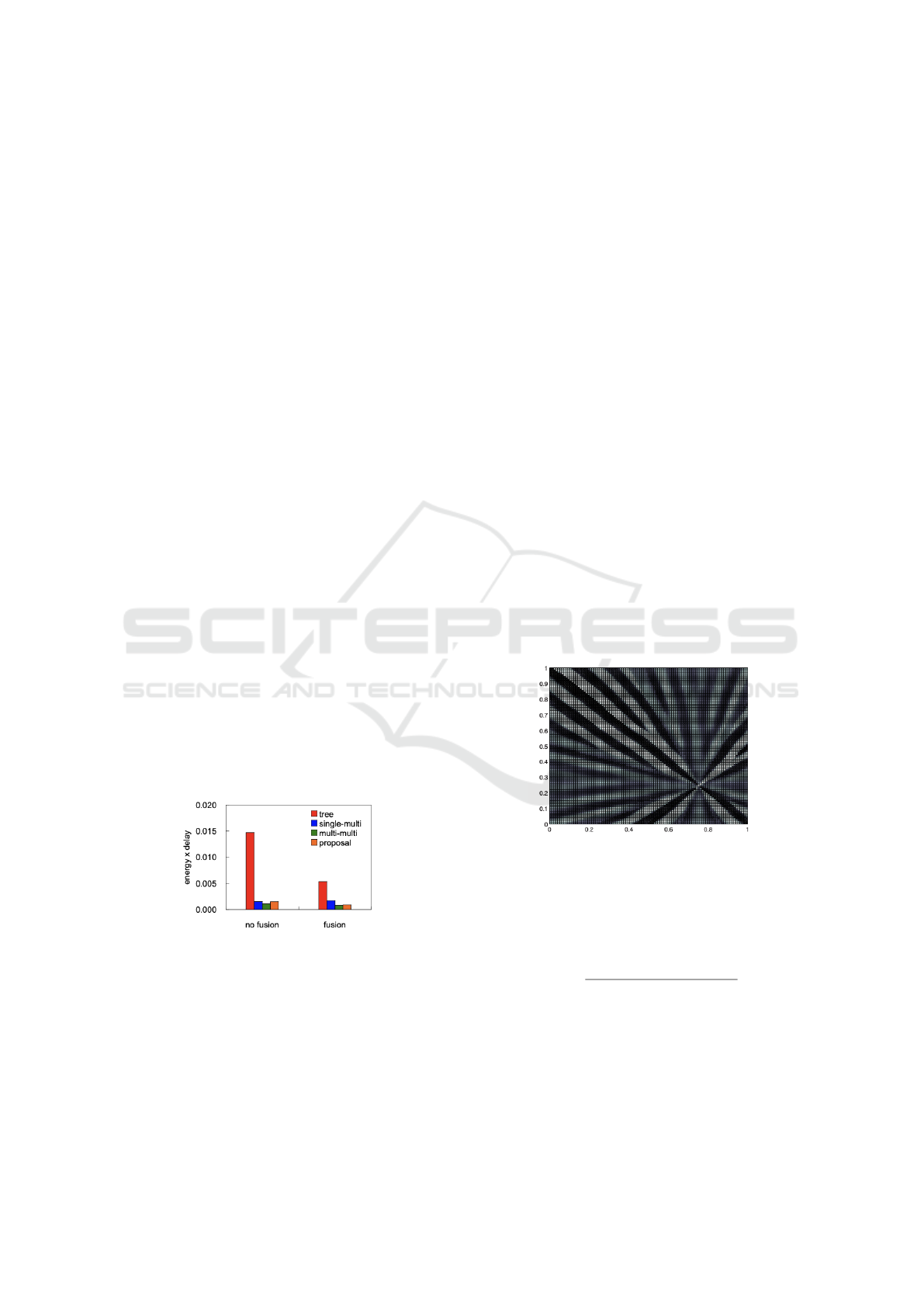
as shown in the Figure 2.
Figure 2: Comparison of topologies in terms of energy effi-
cient and low-delay data gathering (Wakamiya et al., 2008).
4.2 Data Highway for Efficient Routing
Lowe et al. (Lowe and Miorandi, 2009) described a
distributed reaction-diffusion based approach to form
data highways in dense ad hoc wireless sensor net-
works. This approach employed data highways origi-
nated from (Franceschetti et al., 2007), which applied
the Percolation Theory to construct fast-lane paths
for data transmission. Specifically, data highways
are cross-section data transmission paths in a network
that are characterized by the high source-destination
throughput. Such data highways are spatially opti-
mized so every non-highway node is within one hop
away from at least one data highway in the network.
The data highways of a network originally de-
scribed in (Franceschetti et al., 2007) relied on a
prior analysis of the network topology to determine
the highway paths within. To enhance the flexibility
and robustness of the model, Lowe et al. (Lowe and
Miorandi, 2009) used a self-organizing activation-
inhibition diffusion mechanism and the diffusion fil-
ter to determine the optimal data highways through a
WSN.
Consider a WSN where all nodes are under-
lined with variables that denote temporally and spa-
tially varying concentrations of a pair of competing
substances: short-range activator and long-range in-
hibitor. For nodes that will serve as data highways
to emerge, additionally, diffusion filters with the con-
trolled activation axis or orientation are applied so
that stripped patterns or ridges can be generated dur-
ing the diffusion process in the WSN. The orientation
of the diffusion filters also need to be carefully se-
lected so the activation bands are oriented towards the
data sink in the network, such as in Figure 3.
Figure 3: Sensor activation and inhibition with diffusion
filters oriented towards a single data sink (Lowe and Mio-
randi, 2009).
For the WSN with more data sinks, the direction
of the diffusion filter at node N
i
can be given by the
vector D
i
, as follows:
D
i
=
Σ
j∈S
(N
i
− S
j
)|N
i
− S
j
|
−2
Σ
j∈S
|N
i
− S
j
|
−2
(15)
where S is the set of data sinks S
i
.
Once the data highways are generated, each non-
highway node needs to find the closest data highway
by broadcasting until it receives an acknowledge from
a node that belongs to a data highway. The responding
node is then used as an entry point for the broadcast-
ing node to forward its data to the data highway and
Reaction-Diffusion Inspired Sensor Networking: From Theory to Application
235

in turn being relayed to the data sink. Additional op-
timization is required to ensure that data entering the
data highway needs to be routed to the closest and one
data sink only. This is achieved by broadcasting and
exchanging the distance information along nodes on a
given data highway. Numerical experiments provided
in (Lowe and Miorandi, 2009) showed results that are
analogous to the example in Figure 3.
In (Miorandi et al., 2009), Miorandi et al. de-
scribed a refined approach based on (Lowe and Mio-
randi, 2009) to accommodate the fact that all nodes
may not have the perfect information on the rela-
tive locations of data sinks in the WSN. The same
reaction-diffusion-based data highway approach was
used to construct high-throughput data highways.
First, for all nodes to estimate the distance and direc-
tion to data sinks, each data sink broadcasts a beacon
with its ID so all nodes can receive, update and re-
broadcast the distance information.
Second, each node derives its neighborhood by
broadcasting a message to its immediate or one-hop
neighbors in order to learn their one-hop neighbors
until all neighbors located at most R-hop are discov-
ered, along with neighbors’ level of activation.
Third, each node constructs its local activator and
inhibitor regions as its diffusion filter, which will
guide the ridge peak in the activation level to emerge
and orient toward the data sinks. Specifically, for a
given node n
i
, if a neighbor node, n
j
is on the shortest
path to or from a data sink, n
j
therefore is considered
a activator node for the given node. That is: n
i
∈ R
a
where R
a
is the activation region. In contrast, if n
j
is not on the shortest path, n
j
is an inhibitor node, or
n
j
∈ R
i
where R
i
is the inhibition region. The acti-
vation level is updated based on the discrete reaction-
diffusion equation with one activation level variable
u, as follows (Lowe and Miorandi, 2009; Miorandi
et al., 2009):
u(k, t + 1) = g[φ
s
u(k, t)+ Σ
j∈R
i
φ
i
( j)u(k + j,t)+
Σ
j∈R
a
φ
a
( j)u(k + j,t)]
(16)
where k is the location; R
a
and R
i
are the regions
of activation and inhibition respectively; φ
a
, φ
i
, and
φ
s
are coefficients of self-activation, activation, and
inhibition respectively; and g is a normalizing func-
tion. Processes of the second and the third steps are
repeated until a stable pattern is formed.
The approach and the protocols have been im-
plemented and simulated in the event-driven network
simulator, Omnet++ (Varga, 2010). The simulation
showed that using the described approach is able to
construct valid routes (i.e. data highways) to data
sinks. Two performance evaluation metrics are ap-
plied in the simulation. The first is for a given node
the time of acquiring and reaching a valid data high-
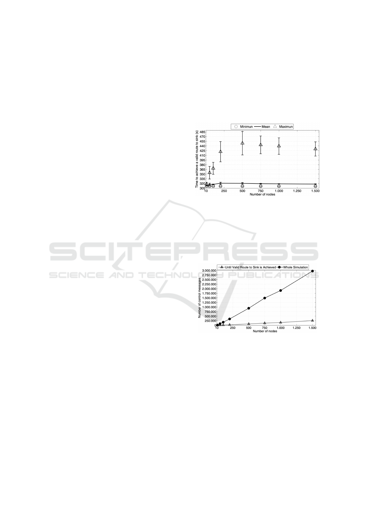
way path to the data sink, which is shown in Figure
4. While the resulting minimum and average time are
slightly sensitive to the number of nodes of the net-
work, the maximum time attained positively depends
on the number of nodes in the network.
Figure 4: Bootstrapping time as a function of the network
size (Miorandi et al., 2009).
The second metric was related to the overhead of
the number of message-exchange needed until reach-
ing a valid data highway to the data sink, as shown in
Figure 5. The result shows that the number of control
messages required increases linearly in the number of
nodes.
Figure 5: Number of Control messages as a function of the
network size (Miorandi et al., 2009).
4.3 Cluster Formation and Cluster
Head Election
In (Yamamoto and Miorandi, 2010) Yamamoto et al.
evaluated two well-known activator-inhibitor mod-
els, Gierer-Meinhardt model and Activator-Substrate
model, on their performance of recovery from pertur-
bation or attacks in the case of the distributed cluster
head computation. The two activator-inhibitor models
are engineered to form spot patterns that correspond
to activator concentration peaks. The location of such
a peak is considered an autonomous processor elected
SENSORNETS 2022 - 11th International Conference on Sensor Networks
236

to execute important commands designated for a clus-
ter head. As a result, the formation of the spot patterns
is much analogous to the cluster head election prob-
lem.
With the goal of preserving the compatible with
future artificial chemistry implementation or natu-
ral chemical computing, such as reaction-diffusion
processors, the approach presented in (Yamamoto
and Miorandi, 2010) first derived the chemical reac-
tions from the reaction terms of the reaction-diffusion
equations for the two models by employing the Law
of Mass Action and considered an additional sub-
stance, the catalyst. The set of chemical reactions
can be described by a system of ordinary differential
equations (ODE), in contrast to the original reaction-
diffusion equations being partial differential equa-
tions (PDE). The chemical reaction system is then
simulated deterministically by integrating the system
of derived ODE from the chemical reactions.
Gierer–Meinhardt activator-inhibitor model
(Gierer and Meinhardt, 1972) is one of the most
widely used activator–inhibitor models. Yamamoto
et al. (Yamamoto and Miorandi, 2010) reverse-
engineered the equations (3) and (4) to derive
corresponding chemical reactions. Similarly a set of
corresponding chemical reactions were derived for
the activator-depleted substrate model (Meinhardt,
1982) and Gray-Scott model (Gray and Scott, 1990).
These three activator-inhibitor based models were
simulated according to the derived chemical reac-
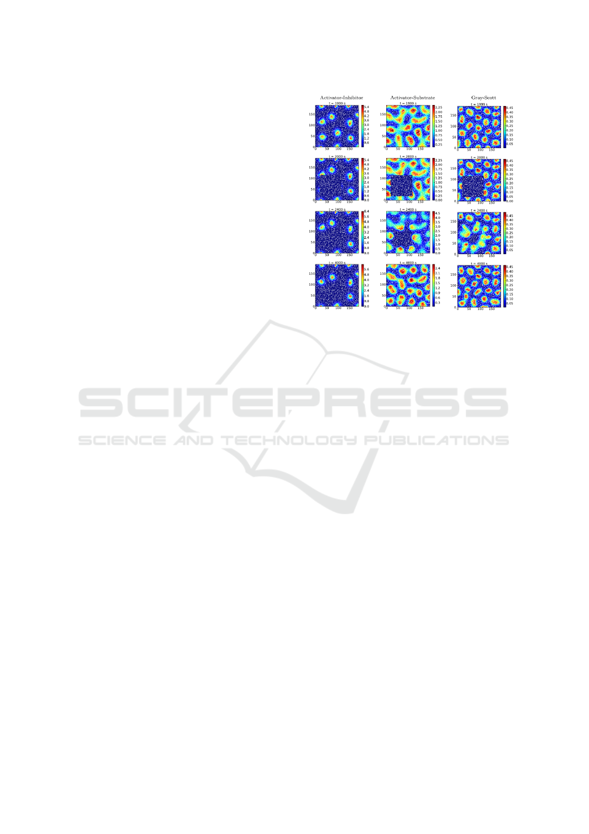
tions. Their experiment results showed a tournament
between the stability of network patterns and the
ability to recover upon disruption. Specifically, for a
method that is more stable with rare failure, it recov-
ers slower from disruption and vice versa as shown
in Figure 6. For instance, The Gierer-Meinhardt
model is more stable, but slower to recover from
disruptions. The activator–substrate model is neutral
that sits between the above two extremities.
Wu et al. (Wu et al., 2020) presented a
Gierer-Meinhardt activator-inhibitor model (Gierer
and Meinhardt, 1972) and G
¨
ur game (Tsetlin, 1973;
Tung and Kleinrock, 1993; Tung, 1994; Tung and
Kleinrock, 1996) based routing algorithm that tries to
reduce the energy consumption of a WSN to max-
imize the network lifetime. The Gierer-Meinhardt
activator-inhibitor model (Gierer and Meinhardt,
1972) is applied for cluster head selection and au-
tonomous clusters formation. Within each cluster, the
G
¨
ur game is to determine the active sensor nodes so
that only the active nodes transmit sensing data to its
cluster head to relay the aggregated data to the base
station.
Figure 6: Recovery behavior of the three reaction–diffusion
models at different time steps: t = 1999 s (before perturba-
tion), t = 2000 s (start to introduce a perturbation), t = 2400
s (recovering), and t = 4000 s (end of simulation). (Ya-
mamoto et al., 2011).
5 CONCLUSION
Since the first reaction-diffusion model had been pro-
posed by Alan Turing in 1952, many subsequent
studies for modeling biological pattern formation
have been proposed. Reaction-diffusion mechanisms
started to gain interest in the research community
of wireless sensor networks researchers about two
decades ago, however it has not yet been widely ap-
plied. In this paper, we gave an overview to the RD
model and introduced three notable activator-inhibitor
based models inspired by the RD model. Selected pa-
pers have been discussed to present the applications of
reaction-diffusion mechanisms in the wireless sensor
networks, including sensor data relaying, data gather-
ing, and cluster formation and cluster head election.
In the RD-based models presented in this pa-
per, we observe that several valuable variant models
that well-suit the algorithmic purposes of assisting
high level computing tasks in WSNs, such as rout-
ing and cluster head election. It is worth of fur-
ther exploring whether there is a trade-off among
various parameters and models when a synergy is
envisioned. Although the mathematical theories of
reaction-diffusion mechanics require sometimes to
narrow parameter choices, the results can be useful
for autonomous systems like sensor fields with dis-
tributed control.
Reaction-Diffusion Inspired Sensor Networking: From Theory to Application
237

REFERENCES
Bar-Yam, Y. (2003). Dynamics of Complex Systems. West-
view Press.
Dressler, F. and Akan, O. B. (2010a). Bio-inspired network-
ing: from theory to practice. IEEE Communications
Magazine, 48(11):176–183.
Dressler, F. and Akan, O. B. (2010b). A survey on bio-
inspired networking. Computer networks, 54(6):881–
900.
Franceschetti, M., Dousse, O., Tse, D. N., and Thiran, P.
(2007). Closing the gap in the capacity of random
wireless networks via percolation theory. IEEE Trans-
actions on Information Theory, 53(ARTICLE):1009–
1018.
Gierer, A. and Meinhardt, H. (1972). A theory of biological
pattern formation. Kybernetik, 12(1):30–39.
Gray, P. and Scott, S. K. (1990). Chemical oscillations and
instabilities: non-linear chemical kinetics. Oxford:
Oxford Science.
Henderson, T. C., Luthy, K., and Grant, E. (2014).
Reaction-diffusion computation in wireless sensor
networks. Jounral of Unconventional Computing.
Henderson, T. C., Venkataraman, R., and Choikim, G.
(2004). Reaction-diffusion patterns in smart sen-
sor networks. In IEEE International Conference
on Robotics and Automation, 2004. Proceedings.
ICRA’04. 2004, volume 1, pages 654–658. IEEE.
Hyodo, K., Wakamiya, N., Nakaguchi, E., Murata, M.,
Kubo, Y., and Yanagihara, K. (2007). Experiments
and considerations on reaction-diffusion based pattern
generation in a wireless sensor network. In 2007 IEEE
International Symposium on a World of Wireless, Mo-
bile and Multimedia Networks, pages 1–6. IEEE.
Kondo, S. and Asai, R. (1995). A reaction–diffusion wave
on the skin of the marine angelfish pomacanthus. Na-
ture, 376(6543):765–768.
Lowe, D. and Miorandi, D. (2009). All roads lead to rome:
Data highways for dense wireless sensor networks. In
International Conference on Sensor Systems and Soft-
ware, pages 189–205. Springer.
Meinhardt, H. (1982). Models of biological pattern forma-
tion. Academic Press, London.
Miorandi, D., Lowe, D., and Gomez, K. M. (2009).
Activation–inhibition–based data highways for wire-
less sensor networks. In International Conference
on Bio-Inspired Models of Network, Information, and
Computing Systems, pages 95–102. Springer.
Nakano, T. (2010). Biologically inspired network systems:
A review and future prospects. IEEE Transactions on
Systems, Man, and Cybernetics, Part C (Applications
and Reviews), 41(5):630–643.
Nakas, C., Kandris, D., and Visvardis, G. (2020). Energy
efficient routing in wireless sensor networks: a com-
prehensive survey. Algorithms, 13(3):72.
Pearson, J. E. (1993). Complex patterns in a simple system.
Science, 261(5118):189–192.
Ren, H. and Meng, M. Q.-H. (2006). Biologically inspired
approaches for wireless sensor networks. In 2006 In-
ternational Conference on Mechatronics and Automa-
tion, pages 762–768. IEEE.
Singh, A., Sharma, S., and Singh, J. (2021). Nature-
inspired algorithms for wireless sensor networks: A
comprehensive survey. Computer Science Review,
39:100342.
Tsetlin, M. (1973). Automaton theory and modeling of bio-
logical systems: by ML Tsetlin. Translated by Scitran
(Scientific Translation Service)., volume 102. Aca-
demic Press.
Tung, B. and Kleinrock, L. (1993). Distributed control
methods. In High Performance Distributed Comput-
ing, 1993., Proceedings the 2nd International Sympo-
sium on, pages 206–215. IEEE.
Tung, B. and Kleinrock, L. (1996). Using finite state au-
tomata to produce self-optimization and self-control.
Parallel and Distributed Systems, IEEE Transactions
on, 7(4):439–448.
Tung, Y.-C. (1994). Distributed control using finite state
automata.
Turing, A. M. (1952). The chemical basis of morphogen-
esis. Philosophical Transactions of the Royal Society
of London. Series B, Biological Sciences, 237(64):37–
72.
Varga, A. (2010). Omnet++. In Modeling and tools for
network simulation, pages 35–59. Springer.
Wakamiya, N., Hyodo, K., and Murata, M. (2008).
Reaction-diffusion based topology self-organization
for periodic data gathering in wireless sensor net-
works. In 2008 Second IEEE International Confer-
ence on Self-Adaptive and Self-Organizing Systems,
pages 351–360. IEEE.
Wu, S.-Y., Brown, T., and Wang, H.-T. (2020). A reaction-
diffusion and g
¨
ur game based routing algorithm for
wireless sensor networks. In International Conference
on Mobile, Secure, and Programmable Networking,
pages 223–234. Springer.
Yamamoto, L. and Miorandi, D. (2010). Evaluating the ro-
bustness of activator-inhibitor models for cluster head
computation. In International Conference on Swarm
Intelligence, pages 143–154. Springer.
Yamamoto, L., Miorandi, D., Collet, P., and Banzhaf, W.
(2011). Recovery properties of distributed cluster
head election using reaction–diffusion. Swarm Intel-
ligence, 5(3):225–255.
Zheng, C. and Sicker, D. C. (2013). A survey on bio-
logically inspired algorithms for computer network-
ing. IEEE Communications Surveys & Tutorials,
15(3):1160–1191.
SENSORNETS 2022 - 11th International Conference on Sensor Networks
238