Application of Sequential Neural Networks to Predict the Approximation

Degree of Decision-making Systems

Jarosław Szkoła

1 a

and Piotr Artiemjew

2 b

The Department of Computer Science, University of Rzeszow, 35-310 Rzeszow, Poland

Faculty of Mathematics and Computer Science, University of Warmia and Mazury in Olsztyn, Poland

Keywords:

Rough Sets, Granulation of Knowledge, Rough Inclusions, Standard Granulation, Estimation of the Approxi-

mation Degree, Sequential Neural Networks.

Abstract:

The paradigm of granular computing appeared from an idea proposed by L. A Zadeh, who assumed that a key

element of data mining techniques is the grouping of objects using similarity measures. He assumed that sim-

ilar objects could have similar decision classes. This assumption also guides other scientiﬁc streams such as

reasoning by analogy, nearest neighbour method, and rough set methods. This assumption leads to the implica-

tion that grouped data, (granules) can be used to reduce the volume of decision systems while preserving their

classiﬁcation efﬁciency - internal knowledge. This hypothesis has been veriﬁed in practice - including in the

works of Polkowski and Artiemjew (2007 - 2015) - where they use rough inclusions proposed by Polkowski

and Skowron as an approximation tool - using the approximation scheme proposed by Polkowski. In this work,

we present the application of sequential neural networks to estimate the degree of approximation of decision

systems (the degree of reduction in the size) based on the degree of indiscernibility of the decision system. We

use the standard granulation method as a reference method. Pre-estimation of the degree of approximation is

an important problem for the considered techniques, in the context of the possibility of their rapid application.

This estimation allows the selection of optimal parameters without the need for a classiﬁcation process.

1 INTRODUCTION

1.1 A Few Words of Introduction to

Rough Set Theory and Granular

Computing

As the basic form of collecting knowledge about cer-

tain problems, we use information systems - in the

sense of collecting intelligence needed to solve prob-

lems. The possibility of modelling decision-making

processes is provided by indiscernibility relations,

see (Pawlak, 1992) We deﬁne an information sys-

tem (Pawlak, 1992) as In f Sys = (Uni, Attr), where

Uni is the universe of objects, Attr the set of at-

tributes describing the objects. We assume that U ni

and Attr are ﬁnite and nonempty. Attributes a ∈

Atr describe the objects of the universe by means

of certain values from their domain (V

) - that is,

a : U → V

. By adding some expert decisions (prob-

lem solutions) to the information system, we obtain

https://orcid.org/0000-0002-6043-3313

https://orcid.org/0000-0001-5508-9856

a decision system that can be deﬁned as a triple

DecSys(Uni, Attr, dec), where dec 6∈ Attr. Problems

u, v ∈ Uni are B–indiscernible whenever a(u) = a(v)

for every a ∈ B, for each attribute set B. This assump-

tion is modelled by indiscernibility relation IND(B).

(u, v) ∈ IND(B) iff a(u) = a(v) for each a ∈ B.

The IND(B) relation divides the universe of objects

into classes

[u]

= {v ∈ Uni : (u, v) ∈ IND(B)},

Deﬁned classes form B-primitive granules, collec-

tions over In f Sys. Connections of primitive granules

form elementary granules of knowledge. The descrip-

tor language (Pawlak, 1992) is used to describe infor-

mation systems, where a descriptor is deﬁned as (a, v)

with a ∈ Attr, v ∈ V

. Formulas are created from the

descriptors using the connectors ∨, ∧, ¬, ⇒. Let us

deﬁne the semantics of formulas, , where [[p]] denotes

the meaning of a formula p:

1. [[(a, v)]] = {u ∈ U : a(u) = v}

2. [[p ∨ q] = [[p]] ∪ [[q]]

3. [[p ∧ q]] = [[p]] ∩ [[q]]

4. [[¬p]] = U \ [[p]].

(1)

984

Szkoła, J. and Artiemjew, P.

Application of Sequential Neural Networks to Predict the Approximation Degree of Decision-making Systems.

DOI: 10.5220/0010992300003116

In Proceedings of the 14th International Conference on Agents and Artiﬁcial Intelligence (ICAART 2022) - Volume 3, pages 984-989

ISBN: 978-989-758-547-0; ISSN: 2184-433X

Objects of the universe Uni in attribute terms B are

described by a feature vector in f

(u) = {(a = a(u)) :

a ∈ B}

1.2 Theoretical Introduction to the

Reference Graulation Method

The paradigm of granular computing in the context

of approximate reasoning was proposed by Zadeh

in (Zadeh, 1979) and has been naturally incorpo-

rated into the rough sets paradigm - see (Lin, 2005),

(L. Polkowski, 2001), (L.Polkowski, 1999), (Skowron

and Stepaniuk, 2001).

One direction in the development of granulation

methods in the context of rough sets has been the

use of rough inclusions, formally derived from the

paradigm of rough mereology see (L. Polkowski,

2001), (L.Polkowski, 1999), (Polkowski, 2005),

(Polkowski, 2006).

In this particular work we will consider one of the

approximate inclusions derived from Łukasiewicz t–

norm. Considering a given system (Uni, Attr), the

rough inclusion µ

(u, v, r) is deﬁned by means of the

formula,

(u, v, r) ⇔

|IND(u, v)|

|Attr|

≥ r

IND(u, v) = {a ∈ Attr : a(u) = a(v)}

The formula µ

(u, v, r) deﬁnes a collection of objects

indiscernible from the central object at some ﬁxed de-

gree r (radius of granulation). The granulation idea

that we use in this work as a base method was pro-

posed by Polkowski in (Polkowski, 2005). It con-

sists in forming for the In f Sys a collection of gran-

ules Gr = mathcalG(Uni), with which the whole uni-

verse of objects Uni is covered, by forming a collec-

tion Cov(U) according to a ﬁxed strategy Str. For

each granule g ∈ Cov(Uni), and each attribute a ∈ A,

a value a(g) = S {a(u) : u ∈ g} is determined. The

system is reduced in size as determined by the granu-

lation radius r used and the covering strategy. We use

majority voting as a reference strategy when forming

objects from granules see (Duda et al., 2000).

The hypothesis that information systems can be

approximated by rough inclusions according to the

described scheme - (Polkowski, 2005) - has been ver-

iﬁed in many works by Polkowski and Artiemjew, in-

cluding (Polkowski, 2015).

1.3 Goal of This Work

In this work, we use Polkowski’s approximation

method (standard granulation) as a reference method

to check the possibility of estimating the degree of ap-

proximation (percentage of reduction of decision sys-

tems). For the estimation, we used the internal de-

gree of r-indiscernibility computed as the number of

combinations without repetition of system objects r-

indiscernible from each other - similar at least in de-

gree r. To achieve our goal, we used sequential neural

networks; we used the naive forecasting method as a

reference method. Our aim was not to ﬁnd the best

existing technique, but to test the initial possibility of

modelling the problem under study.

The rest of the paper is organised as follows. Sect.

2 contains the methodology. Sect. 3 contains the re-

sults of experiments. Section 4 contain the conclu-

sions and future works.

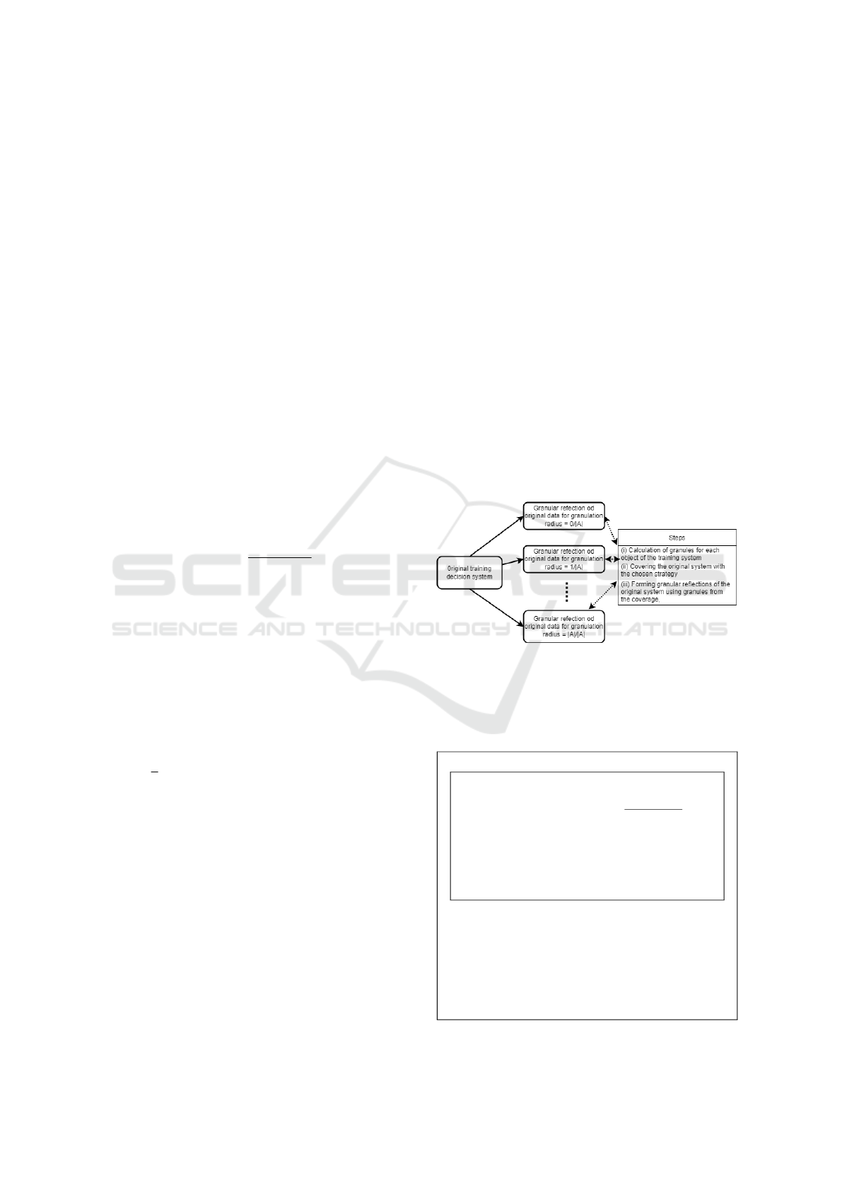
Let us move on to present a toy example of cre-

ating a granular reﬂection of a decision system using

standard granulation (see Fig. 1).

2 RESEARCH METHODOLOGY

Figure 1: In the ﬁgure we have a brief demonstration of the

standard granulation process.

2.1 Standard Granulation - Toy

Example

Assuming that g

gran

) = {u

∈U

trn

|IND(u

, u

|A|

≥ r

gran

}

IND(u

, u

) = {a ∈ A;a(u

) = a(u

)}

trn

is the universe of training objects,

and |X| is the cardinality of set

The sample standard granules with a 0.25

radius, derived from decision systems from Tab.

1 look as follows,

0.25

) = {u

, }

0.25

) = {u

, u

, }

0.25

) = {u

, u

, }

Application of Sequential Neural Networks to Predict the Approximation Degree of Decision-making Systems

985

0.25

) = {u

, u

, }

0.25

) = {u

, }

0.25

) = {u

, u

, }

0.25

) = {u

, }

0.25

) = {u

, u

, }

0.25

) = {u

, }

0.25

) = {u

, u

, }

Random coverage of training systems is as

follows, Cover(U

trn

) = {g

0.25

), g

0.25

), g

0.25

), g

0.25

), g

0.25

), }

To summarise, the example described is the granula-

tion of system from Tab. 1, as an assisting granularity

tool array from Tab. 2 is used. The granular reﬂection

of the original system is in the Tab. 3.

Table 1: Exemplary decision system: diabetes, 9 attributes,

10 objects.

Day a1 a2 a3 a4 a5 a6 a7 a8 class

6 148 72 35 0 33.6 0.627 50 1

1 85 66 29 0 26.6 0.351 31 0

8 183 64 0 0 23.3 0.672 32 1

1 89 66 23 94 28.1 0.167 21 0

0 137 40 35 168 43.1 2.288 33 1

5 116 74 0 0 25.6 0.201 30 0

3 78 50 32 88 31.0 0.248 26 1

10 115 0 0 0 35.3 0.134 29 0

2 197 70 45 543 30.5 0.158 53 1

8 125 96 0 0 0.0 0.232 54 1

Table 2: Triangular indiscernibility matrix for stan-

dard granulation (i < j), derived from Tab. 1 c

i j

1, i f

|IND(u

|A|

≥ 0.25 and d(u

) = d(u

), 0, otherwise.

1 0 0 0 0 0 0 0 0 0

x 1 0 1 0 0 0 0 0 0

x x 1 0 0 1 0 1 0 1

x x x 1 0 0 0 0 0 0

x x x x 1 0 0 0 0 0

x x x x x 1 0 1 0 1

x x x x x x 1 0 0 0

x x x x x x x 1 0 1

x x x x x x x x 1 0

x x x x x x x x x 1

Let us now turn to the introduction of the architec-

ture and description of the sequential neural network

used to achieve the goal of the work.

Table 3: Standard granular reﬂection of the exemplary train-

ing system from Tab. 1, in radius 0.25, 9 attributes, 6 ob-

jects; MV is Majority Voting procedure (the most frequent

descriptors create a granular reﬂection).

Day a1 a2 a3 a4 a5 a6 a7 a8 class

MV (g

0.25

)) 6 148 72 35 0 33.6 0.627 50 1

MV (g

0.25

)) 1 85 66 29 0 26.6 0.351 31 0

MV (g

0.25

)) 0 137 40 35 168 43.1 2.288 33 1

MV (g

0.25

)) 3 78 50 32 88 31.0 0.248 26 1

MV (g

0.25

)) 8 183 64 0 0 23.3 0.672 32 1

MV (g

0.25

)) 2 197 70 45 543 30.5 0.158 53 1

2.2 Forecasting using a Sequential

Neural Network

We used the MSE (Mean Square Error) parameter

to estimate the quality of the presented forecasting

method. Which, when comparing these parameters

on speciﬁc data, is an objective solution.

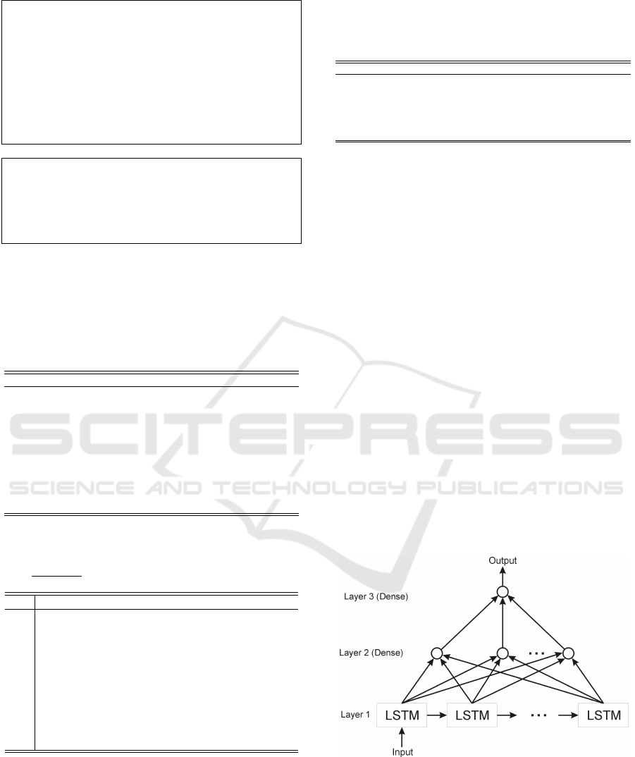
The three-layer sequential neural network archi-

tecture (Szkoła et al., 2011) (Szkola et al., 2011) (Li

et al., 2020) was proposed for predicting the output

data, the ﬁrst layer contains LSTM cells, in subse-

quent layers full connections between the preceding

layer and the current one. In the ﬁrst layer, was used

from 50 to 100 neurons for different input datasets, in

the second layer 25 and in the last layer - one neu-

ron. This conﬁguration works well in most cases of

the input datasets. To obtain a sufﬁciently high qual-

ity of prediction, number of neurons in the network

should be carfully selected. After many attempts, we

can recommend using 2 - 5 times more neurons in

the ﬁrst layer than the input time samples of the data

from the individual time steps. With this range of in-

put neurons, we could achieve good balans beetwen

genralization and overﬁting.

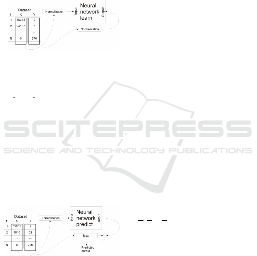
Before the learning process begins, the input data

must be properly processed to the form in which

learning can take place (Szkoła et al., 2011). The

input data supplied to the network should be in the

range in which the training algorithms based on gradi-

ent methods do not cause rapid saturation. In practice,

the input data is converted to the range [0 - 1] or [-1,

ICAART 2022 - 14th International Conference on Agents and Artiﬁcial Intelligence

986

1]. The presented algorithm uses the method of nor-

malizing the input and output data separately, to the

range of values [0 - 1]. Attempts were also made to

transform the input data by means of logarithmic nor-

malization, but it did not improve the classiﬁcation /

prediction of the data, therefore it was decided that

the classical normalizing algorithm would be used.

The learning process involves the sequential feed-

ing of individual samples to the input of the net-

work, based on a method known as online learning

(batch size = 1). The network is learned through

1000 epochs, if less epochs was used, accuracy

was lower value. As the loss function is used

mean squared error, the optimizer used is the Adap-

tive Moment Estimation algorithm.

A simple pre-processing and post-processing op-

eration was used to match the network response to the

expected output values (Szkoła and Pancerz, 2019).

For the input data we used normalization algorithm.

For the compute output value, in the ﬁrst step, the

maximum value that is possible on the output for the

training data is calculated. Then this value is multi-

plied by the network response to the given excitation,

as a result of which we obtain the predicted response

in the range of values consistent with the input data.

Due to the range of values that the network can re-

turn, it is not possible to obtain the target value di-

rectly from the network, therefore a simple operation

of multiplying the network response by an appropri-

ate factor is required.

The number of neurons in the ﬁrst layer has a great

inﬂuence on the correct operation of the network. The

number of neurons in this layer should be greater than

the number of data records. The tests show that good

results are obtained if the number of the neurons in

the ﬁrst layer is at least two or more times greater than

the number of input records. Changes in the number

of neurons in the next layer have a smaller impact on

the functioning of the network.

MSE =

number o f data points

∑

i=1

(observed

− predicted

)

Let us move on to discuss the experimental veriﬁ-

cation of the objective deﬁned in Sect. 1.3.

3 EXPERIMENTAL SESSION

3.1 Data Preparation

For the experiments, we selected a few distinctly dif-

ferent datasets from the UCI repository (Dua and

Graff, 2017).

(i) Australian Credit (dims.: 15, items: 690);

(ii) Car (dims.: 7, items: 1728);

(iii) Congressional house votes (dims.: 17, items:

435);

(iv) Fertility (dims.: 10, items: 100);

(v) German credit (dims.: 20, items: 1000);

(vi) Heart Disease (dims.: 14, items: 270);

(vii) Pima Indians Diabetes (dims.: 9, items: 768).

(viii) Soybean large (dims.: 36, items: 683);

(ix) SPECTF (dims.: 45, items: 267);

(x) SPECT (dims.: 23, items: 267);

For simplicity in the standard granulation process,

all attributes are treated as symbolic.

3.2 Results Description

For the Australian Credit Dataset. Consid-

ering the granulation (approximation) radii as:

{

|A|

, ...,

|A|

}, the size of the granulated (approx-

imated) systems is as follows:1 1 2 3 4 9 24 67

141 355 551 663 682 684 690. A naive predic-

tion solution applying the previous step to the eval-

uation gives an estimate: 1 2 3 5 7 13 33 91 208

496 906 1214 1345 1366 1374. Finally our sequen-

tial neural network which is based on indiscernibil-

ity degrees 237705 237360 233062 215300 178050

125809 73344 33300 10990 2432 351 42 18 9 0 gives

an estimate: 2.954362 -1.041474 0.421173 0.848999

1.51634 5.706955 19.51853 62.379723 138.676437

353.199066 550.998535 660.025024 684.502258

687.227844 686.925232. Calculating the MSE, for

the naive solution is 1827233, and for our approach

Application of Sequential Neural Networks to Predict the Approximation Degree of Decision-making Systems

987

done with a sequential neural network is around 117.

The exact data on which the neural network worked

can be seen in Tab 4.

Table 4: Data for Australian Credit Diabetes: In the table

we have summary information about the values used by the

neural network (input), the expected values, and the values

predicted by the network.

input expected predicted

237705.000000 0.000000 2.954362

237360.000000 0.000000 -1.041474

233062.000000 1.001451 0.421173

215300.000000 2.002903 0.848999

178050.000000 3.004354 1.516340

125809.000000 8.011611 5.706955

73344.000000 23.033382 19.518530

33300.000000 66.095791 62.379723

10990.000000 140.203193 138.676437

2432.000000 354.513788 353.199066

351.000000 550.798258 550.998535

42.000000 662.960813 660.025024

18.000000 681.988389 684.502258

9.000000 683.991292 687.227844

0.000000 690.000000 686.925232

For the Pima Indians Diabetes Dataset. The size

of the granulated systems is as follows:1 23 122 393

633 757 768 768 768. A naive prediction solution:

1 24 145 515 1026 1390 1525 1536 1536. Finally

our sequential neural network gives an estimate: 7.4e-

05 22.028669 121.157761 392.511017 632.823975

756.985718 768 767.999939 768. Calculating the

MSE, for the naive solution is 2323249, and for our

approach done with a sequential neural network is

around 3. The exact data on which the neural network

worked can be seen in Tab 5.

Table 5: Data for Pima Indians Diabetes: In the table we

have summary information about the values used by the

neural network (input), the expected values, and the values

predicted by the network.

input expected predicted

294528.000000 0.000000 0.000074

115994.000000 22.028683 22.028669

38060.000000 121.157757 121.157761

5271.000000 392.511082 392.511017

375.000000 632.823990 632.823975

13.000000 756.985658 756.985718

0.000000 768.000000 768.000000

0.000000 768.000000 767.999939

0.000000 768.000000 768.000000

For the Heart Disease Dataset. The size of the

granulated systems is as follows:1 1 3 3 8 12 25

63 135 214 261 270 270 270. A naive predic-

tion solution: 1 2 4 6 11 20 37 88 198 349 475

531 540 540. Finally our sequential neural net-

work gives an estimate: 2.384996 1.747474 5.694103

4.539211 7.185006 16.565092 35.658192 74.358444

142.456848 216.848175 255.135269 260.954498

261.508392 263.523743 Calculating the MSE, for the

naive solution is 282764, and for our approach done

with a sequential neural network is around 570. The

exact data on which the neural network worked can

be seen in Tab 6.

Table 6: Data for Heart Disease: In the table we have sum-

mary information about the values used by the neural net-

work (input), the expected values, and the values predicted

by the network.

input expected predicted

36315.000000 0.000000 2.384996

36160.000000 0.000000 1.747474

35035.000000 2.007435 5.694103

31203.000000 2.007435 4.539211

24157.000000 7.026022 7.185006

15514.000000 11.040892 16.565092

7882.000000 24.089219 35.658192

3016.000000 62.230483 74.358444

780.000000 134.498141 142.456848

137.000000 213.791822 216.848175

10.000000 260.966543 255.135269

0.000000 270.000000 260.954498

0.000000 270.000000 261.508392

0.000000 270.000000 263.523743

For the rest of the examined data, we only present

the calculated MSE values, which can be seen in the

summary - see Tab. 7.

3.3 Summary of the Results

The results in Tab. 7 show the great advantage of

forecasting with a sequential neural network over the

naive method. Our method allows us to estimate the

degree of approximation (expected reduction of the

original decision systems) in a reasonably accurate

way. The goal we set in section 1.3 has been achieved.

It is worth noting that the estimation presented is a

preview of the possibility of estimating the approxi-

mation degrees and there is a slight overﬁtting process

on the examined data. The only way to compensate

for this process was to select an appropriate neural

network structure. Certainly, the possibility of esti-

mating successive degrees of approximation is higher

than the efﬁciency of the naive method.

ICAART 2022 - 14th International Conference on Agents and Artiﬁcial Intelligence

988

Table 7: Summary results of the efﬁciency of predicting the

size of granular systems vs the efﬁciency of a naive solua-

tion. A smaller MSE value means better prediction preci-

sion.

dataset MSE naive MSE of neural network

Australian credit 1827233 117

Pima Indians Diabetes 2323249 3

Heart disease 282764 570

Car 126860 133

Fertility 13879 11

German credit 4732593 2239

Hepatitis 108585 789

Congressional house votes 42254 780

Soybean large 477873 6786

SPECT 78780

SPECTF 2596795 116

4 CONCLUSIONS

In this ongoing work, we veriﬁed that it is possible to

predict the degree of approximation of decision sys-

tems based on their internal degree of indiscernibil-

ity. To achieve this goal, we used sequential neural

networks, whose efﬁciency proved statistically supe-

rior to the naive prediction method. In the initial es-

timation model used, we are aware of a slight overﬁt-

ting process due to the characteristics of the data se-

quences used. Despite promising initial results, much

is left to be done to evaluate the ﬁnal performance

and determine the application of this new method.

The discovery of the ability to estimate approxima-

tion degrees described in the paper opens up several

new research threads. First, we intend to investigate

whether the estimated degrees allow us to estimate the

behaviour of decision systems in a double granula-

tion process. That is, to verify whether the optimal

approximation parameters can be directly estimated

from the degrees of indiscernibility of the decision

systems. Another horizon of potential research is to

try estimating the course of the approximation on pre-

viously unseen data based on other data with a similar

degree of indiscernibility.

REFERENCES

Dua, D. and Graff, C. (2017). UCI machine learning repos-

itory.

Duda, R. O., Hart, P. E., and Stork, D. G. (2000). Pat-

tern Classiﬁcation (2nd Edition). Wiley-Interscience,

2 edition.

L. Polkowski, A. S. (2001). Rough mereological calculi

of granules: A rough set approach to computation.

Computational Intelligence. An International Journal,

pages 472–492.

Li, G., Xu, J., Shen, W., Wang, W., Liu, Z., and Ding, G.

(2020). Lstm-based frequency hopping sequence pre-

diction. In 2020 International Conference on Wire-

less Communications and Signal Processing (WCSP),

pages 472–477.

Lin, T. (2005). Granular computing: examples, intuitions

and modeling. In 2005 IEEE International Confer-

ence on Granular Computing, volume 1, pages 40–44.

L.Polkowski, A. (1999). Towards an adaptive calculus of

granules. In: L.A.Zadeh, J.Kacprzyk (Eds.), Comput-

ing with Words in Information/Intelligent Systems 1.,

Physica Verlag, pages 201–228.

Pawlak, Z. (1992). Rough Sets: Theoretical Aspects of

Reasoning about Data. Kluwer Academic Publishers,

USA.

Polkowski, L. (2005). Formal granular calculi based on

rough inclusions. pages 57–62. In Proceedings of the

2005 IEEE Conference on Granular Computing.

Polkowski, L. (2006). A model of granular computing with

applications. granules from rough inclusions in infor-

mation systems. pages 9 – 16.

Polkowski, L.; Artiemjew, P. (2015). Granular Computing

in Decision Approximation - An Application of Rough

Mereology. Springer: Cham, Switzerland.

Skowron, A. and Stepaniuk, J. (2001). Information gran-

ules: Towards foundations of granular computing. Int.

J. Intell. Syst., 16:57–85.

Szkoła, J. and Pancerz, K. (2019). Pattern recognition in se-

quences using multistate sequence autoencoding neu-

ral networks. In 2019 International Conference on In-

formation and Digital Technologies (IDT), pages 443–

448.

Szkoła, J., Pancerz, K., and Warchoł, J. (2011). A bezier

curve approximation of the speech signal in the clas-

siﬁcation process of laryngopathies. In 2011 Feder-

ated Conference on Computer Science and Informa-

tion Systems (FedCSIS), pages 141–146.

Szkoła, J., Pancerz, K., and Warchoł, J. (2011). Recurrent

neural networks in computer-based clinical decision

support for laryngopathies: An experimental study.

Intell. Neuroscience, 2011.

Szkola, J., Pancerz, K., Warchol, J., Babiloni, F., Fred, A.,

Filipe, J., and Gamboa, H. (2011). Improving learn-

ing ability of recurrent neural networks-experiments

on speech signals of patients with laryngopathies. In

BIOSIGNALS, pages 360–364.

Zadeh, L. (1979). Fuzzy sets and information granularity.

Technical Report UCB/ERL M79/45, EECS Depart-

ment, University of California, Berkeley.

Application of Sequential Neural Networks to Predict the Approximation Degree of Decision-making Systems

989