
Semi-automatic CNN Architectural Pruning using the Bayesian Case
Model and Dimensionality Reduction Visualization
Wilson E. Marc
´
ılio-Jr.
1 a
, Danilo M. Eler
1 b
and Ivan R. Guilherme
2 c
1
Department of Mathematics and Computer Science, S
˜
ao Paulo State University - UNESP, Presidente Prudente, SP, Brazil
2
Department of Statistics, Applied Math. and Computing, S
˜
ao Paulo State University - UNESP, Rio Claro, SP, Brazil
Keywords:
CNN Pruning, Case-based Reasoning, Visualization.
Abstract:
Visualization techniques have been applied to reasoning about complex machine learning models. These vi-
sual approaches aim to enhance the understanding of black-box models’ decisions or guide in hyperparameters
configuration, such as the number of layers and neurons/filters in deep neural networks. While several works
address the architectural tuning of convolutional neural networks (CNNs), only a few works face the problem
from a semi-automatic perspective. This work presents a novel application of the Bayesian Case Model that
uses visualization strategies to convey the most important filters of convolutional layers for image classifica-
tion. A heatmap coordinated with a scatterplot visualization emphasizes the filters with the most contribution
to the CNN prediction. Our methodology is evaluated on a case study using the MNIST dataset.
1 INTRODUCTION
Visualization techniques play a major role in under-
standing the learning patterns of deep neural networks
due to their low interpretation abilities. For example,
visual approaches are created to enhance understand-
ing of how convolutional neural networks apply series
of non-linear equations to images (Liu et al., 2017a;
Zeiler and Fergus, 2014), how attention mechanisms
can uncover dependencies among words in recur-
rent neural networks (Strobelt et al., 2018), and how
to progressively inspect the training process (Rauber
et al., 2017; Pezzotti et al., 2018; Marcilio-Jr et al.,
2020).
The design of neural networks is usually a time-
consuming task where various decisions, such as the
number of layers, number of neurons in each layer,
and other aspects must be taken into account (Good-
fellow et al., 2016). The decision of these parameters
is usually taken based on the practitioners’ intuition
or various trial-and-error iterations. Usually, the first
step consists of choosing a complex architecture to
perform the learning task. Then, such architecture is
refined so that simpler models could maintain perfor-
mance while requiring a much lower number of pa-
a
https://orcid.org/0000-0002-8580-2779
b
https://orcid.org/0000-0002-9493-145X
c
https://orcid.org/0000-0002-3610-3779
rameters. In particular, the refinement of the architec-
ture is performed by inspecting the model after train-
ing. For example, one could remove all the close to
zero parameters in a feed-forward neural network. To
this end, visualization techniques also play a major
role in understanding the processes involving neural
networks. One beneficial approach is to use Visual
Analytics tools to help define model architecture, as
shown by Garcia et al. (Garcia et al., 2019), that pro-
vides visual metaphors based on heatmaps to uncover
and emphasize filters that could be removed from con-
volutional neural networks.
However, the literature lacks techniques that indi-
cate which filters are prone to be removed from in-
spected layers, i.e., using semi-automatic strategies.
In this scenario, users would benefit from the cues
given by the automatic techniques while assessing
the performance of such cues using visual represen-
tations.
In this work, we propose a novel application of
the Bayesian Case Model (BCM) (Kim et al., 2014)
to uncover the most important convolutional filters
of CNNs applied to image classification. The result
of BCM, which consists of data samples that most
describe datasets, is visualized through a scatterplot-
based visualization after dimensionality reduction,
which has been widely applied to investigate the
learning process of deep learning models (Rauber
et al., 2017; Marc
´
ılio-Jr et al., 2021b; Marc
´
ılio-Jr
E. Marcílio-Jr., W., Eler, D. and Guilherme, I.
Semi-automatic CNN Architectural Pruning using the Bayesian Case Model and Dimensionality Reduction Visualization.
DOI: 10.5220/0010991000003124
In Proceedings of the 17th International Joint Conference on Computer Vision, Imaging and Computer Graphics Theory and Applications (VISIGRAPP 2022) - Volume 3: IVAPP, pages
203-209
ISBN: 978-989-758-555-5; ISSN: 2184-4321
Copyright
c
2022 by SCITEPRESS – Science and Technology Publications, Lda. All rights reserved
203

et al., 2021a). The scatterplot visualization is coordi-
nated with a heatmap summarizing an activation map
that emphasizes which filters could be candidates for
removal. Thus, instead of automatically pruning the
network with the result of BCM, our approach en-
hances the trust in the final refinement by letting the
users decide which filters—among those indicated by
BCM—will be removed from the network. Finally,
our approach is evaluated through a case study on the
classification of the MNIST dataset. Summarily, the
contributions of this paper are:
• Application of the Bayesian Case Model for prun-
ing convolutional neural network;
• A visualization approach for supporting in the net-
work pruning.
This work is organized as follows: in Section 2
we present the related works; Section 3 focus on the
explanation of the Bayesian Case Model; our method-
ology is delineated in Section 4; a use case is provided
in Section 5; discussions about the work are provided
in Section 6; finally, the work is concluded in Sec-
tion 7.
2 RELATED WORKS
Using visualization strategies to understand the
caveats and decisions taken by neural networks has
been a trending topic in the visualization community
in the past few years, mainly due to the need to ex-
plain these complex models.
According to Pezzotti et al. (Pezzotti et al., 2018),
the visualization techniques designed to enhance the
analysis of deep neural networks (DNNs) can be
divided into three groups: weight-centric, dataset-
centric, and filter-centric techniques. The weight-
centric techniques aim at understanding the relation-
ship among the weight learned by the networks so
that the learning process can be understood based
on a combination of input-weight-output. These ap-
proaches use node-link diagrams (Reingold and Til-
ford, 1981), and visual clutter is reduced by neu-
ron aggregation and edge bundle (Liu et al., 2017a).
Dataset-centric techniques are usually employed to
understand the training process of neural networks
from a higher point of view, such as using dimension-
ality reduction algorithms to understand the training
evolution of such techniques (Rauber et al., 2017) or
using star-plots to monitor the evolution of the train-
ing process as well as comparing different deep learn-
ing models (Marcilio-Jr et al., 2020). Finally, filter-
centric methodologies aim to understand the patterns
learned by the filters, for example, by visualizing the
relationships among filters and the labels associated
with them (Rauber et al., 2017). Garcia et al. (Garcia
et al., 2019), for example, use activation maps to com-
municate the filter’s redundancy to help in architec-
tural tuning. Hohman et al. (Hohman et al., 2020) use
aggregation to visualize which features deep learning
models have learned and how these features interact
inside the model to produce predictions. Clavien et
al. (Clavien et al., 2019) utilize heatmap representa-
tions to progressively visualize the neuron’s activation
during the training of deep learning models.
More related to our work are techniques aiming
to reduce models by pruning filters. The majority of
the methods propose automatic approaches that uses
thresholds to remove filters from CNNs (Luo et al.,
2017; Liu et al., 2017b; He et al., 2017; Yu et al.,
2018; Dubey et al., 2018; He et al., 2019). For in-
stance, Li et al. (Li et al., 2021) propose a visual an-
alytics system to provide users with a better view of
the convolutional filters of CNNs and support them
with pruning plans. Thus, our work lies between these
two approaches since we indicate to users which fil-
ters may be good for removal but leave the final to
them the final decision.
This work presents a semi-automatic approach
that uses visualization strategies to help in the ar-
chitectural pruning of convolutional neural networks.
First, we briefly introduce the Bayesian Case Model
(BCM) to explain how it searches for features that ex-
plain clustering results. Then, we introduce our ap-
proach that uses the BCM output to generate hints for
filter removal.
3 BAYESIAN CASE MODEL
The Bayesian Case Model (BCM) (Kim et al., 2014)
is an interpretable model that tries to describe the la-
tent space of a high-dimensional dataset through clus-
ters’ prototypes and their subspaces. These proto-
types (that correspond to actual data points) are de-
scribed by several features that characterize the data
points. In other words, the prototypes are described
by a series of features that are important to them.
BCM execution starts with a standard discrete
mixture model (Hofmann, 1999) to represent the
structure of the data points. Since only the mixture
model cannot interpret the clustering result, in the
sense that which features contribute the most for the
cluster formation, BCM augments the mixture model
result by adding the prototypes and subspace feature
indicators to characterize/explain the clusters. A few
parameters are involved in the BCM execution, as
shown in Fig. 1.
IVAPP 2022 - 13th International Conference on Information Visualization Theory and Applications
204
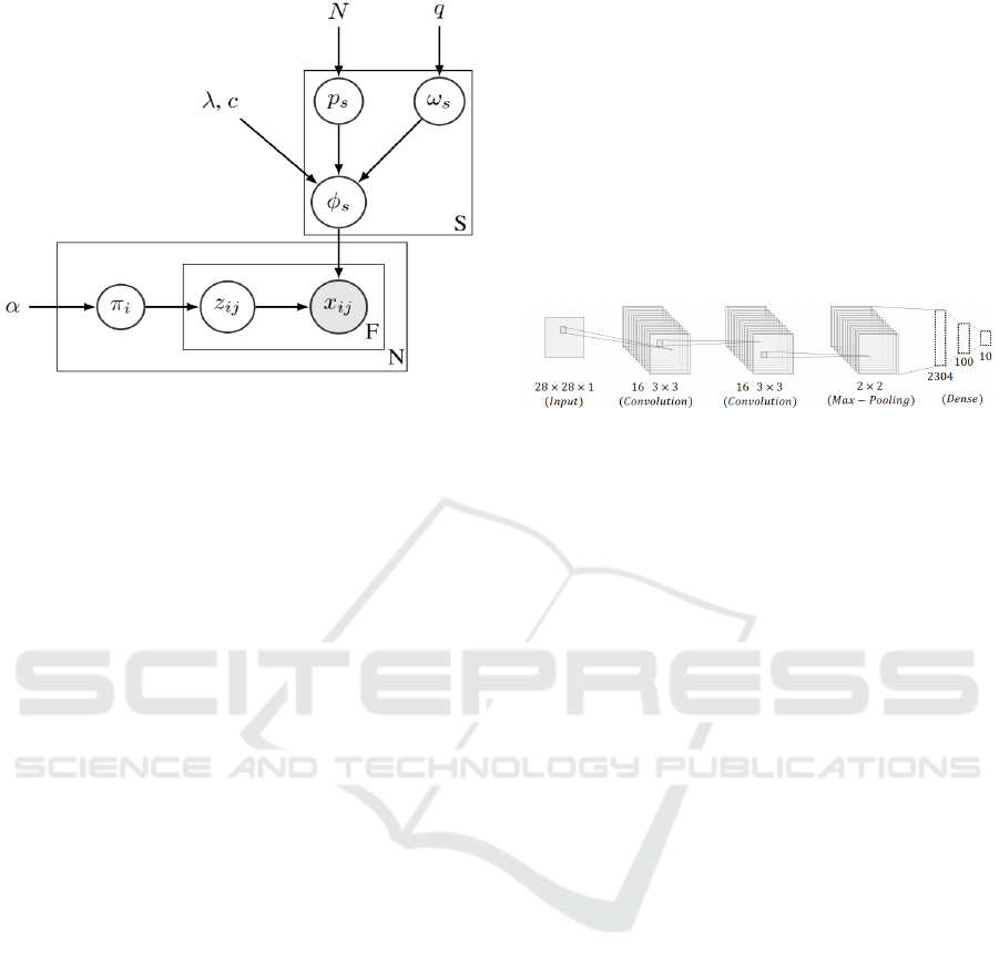
Figure 1: Graphical representation of BCM tecnique (Kim
et al., 2014).
The graphical representation indicates all the com-
ponents used in BCM. Firstly, the algorithm starts
with N observations (X = {x
1
, x
2
, ..., x
N
}), where each
observation (x
i
) represent a random mixture over S
clusters. At the beginning of the algorithm, each data
point is described by each cluster with random contri-
butions. These contributions are indicated in Fig. 1 by
the mixture weights (π
i
∈ R
S
+
) that associate a num-
ber to each data point, denoted by x
i j
. Each of these
features is given from one cluster, meaning that which
cluster (or subspace) contributes the most to defining
the data point. The indication of which cluster defines
feature x
i j
is denoted by z
i j
, and it assumes a value be-
tween 1 and S. The hyper-parameters q, λ, c, and α
are assumed to be fixed.
BCM is trained so that it returns the prototypes
and their corresponding subspaces. While the proto-
types correspond to actual data points, the subspaces
are a way to tell which features contribute the most to
defining the clusters—represented by the prototypes.
A complete description of the BCM training process
is out of the scope of this paper, and interested read-
ers can refer to the original article by Kim et al. (Kim
et al., 2014).
4 METHODOLOGY
Defining the architecture of deep learning models is
usually a process carried out based on the practi-
tioners’ experience. One of the most employed ap-
proaches is to start with a complex model (e.g., too
many layers, neurons, or convolutional filters) and
then refine the architecture while retraining the model
to investigate its ability to generalize well for the data.
In this case, approaches that help machine learning
practitioners to spend less time on architectural tun-
ing are of the great value of rapid prototyping.
Our methodology for architectural tuning is fo-
cused on the convolutional layers of convolutional
neural networks (CNNs). Consider the CNN archi-
tecture of Fig. 2, which we also use in the use case
(see Section 5). After the input, the two convolu-
tional layers are responsible for extracting images’
features. The dense part of the network contains
neurons that use these characteristics to discriminate
among classes.
Figure 2: CNN architecture used to train MNIST dataset.
After the training step, we can input an image to
the convolutional filters to investigate the importance
of that image’s structures. In other words, the con-
volutional process of an input image to the trained
layers will result in values that show how each filter
assigns importance to that input image and its struc-
tures. Given an input dataset X that consists of |X|
images, the set of activation images for an input im-
age X
i
results from applying a convolutional layer l
k
and is denoted as l
k
(X
i
). The application of l
k
to an
input image X
i
returns m activation images, resulted
from convolution of m filters by image X
i
. For exam-
ple, in Fig. 2, the application of layer l
2
to an input
image X
i
(l
2
(X
i
)) results in 16 activation images since
it contains 16 convolutional filters.
For a single input image, our task is to provide the
users with the filters that would be the candidates for
the removal. Thus, we use BCM to return such infor-
mation based on the activation images of that image.
Since BCM accepts a matrix of observations by di-
mensions, we transform the filter activations of each
input image into dimensions. So, we transpose the
matrix of flattened convolutional filters, as shown in
Fig. 3. Before feeding such a matrix to BCM, we
first linearly scale each pixel of filter activation to the
range ∈ [0, 10] to decrease the computing time of the
BCM algorithm. From the output of BCM, we are
only interested in the subspaces, i.e., the features of
the matrix and, consequently, the filters that are most
important for the input images.
Notice that by transposing the matrix of flattened
convolutional filters (see Fig. 3), we construct a ma-
trix in which each filter corresponds to a column. We
choose to represent the filters as columns since BCM
returns prototypes (rows of the matrix) and the asso-
ciated dimensions (columns of the matrix) used to de-
Semi-automatic CNN Architectural Pruning using the Bayesian Case Model and Dimensionality Reduction Visualization
205
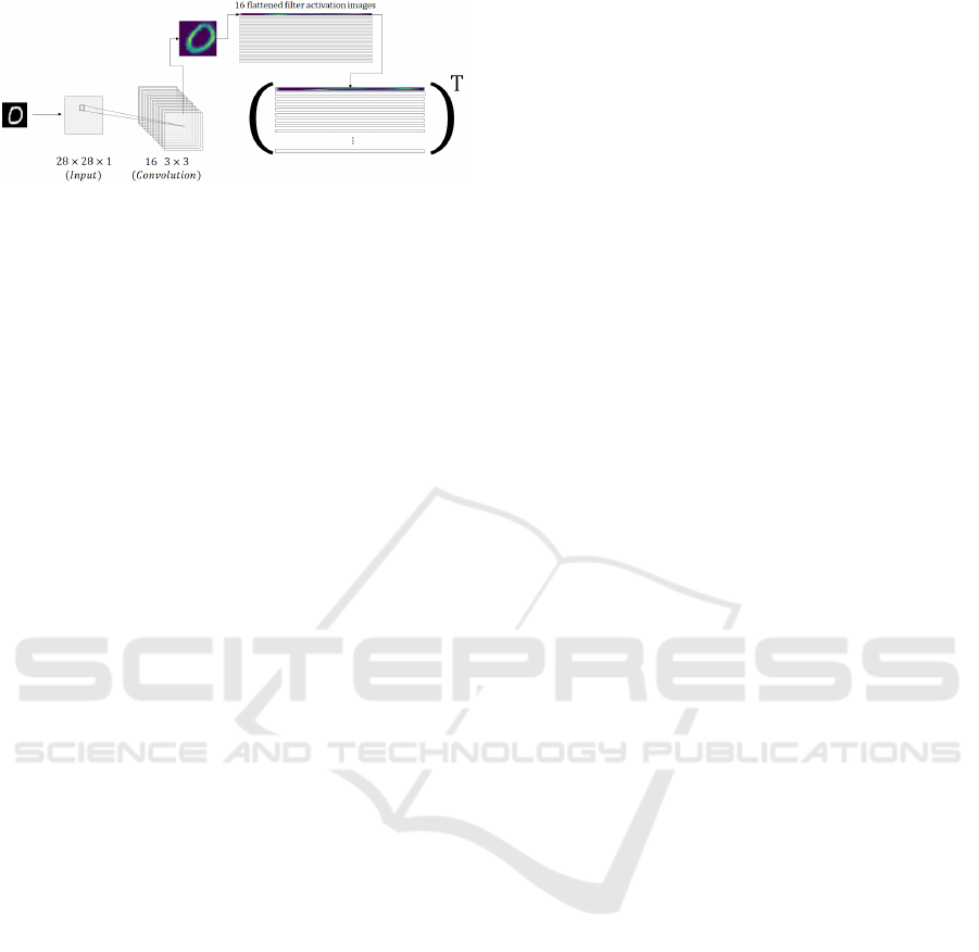
Figure 3: Generating input matrix for BCM technique. For
each input image, m activation images are generated, where
m is the number of filters in the analyzed layer. These acti-
vation images are flattened and then transposed to be fed to
the BCM technique.
scribe the prototype. Thus, choosing only one pro-
totype for the matrix created using the activation im-
ages of an input image, BCM returns the dimensions
used to describe all of the matrices, in other words,
the most important filters. We discard the prototype
in our application.
Finally, since we have to repeat the process de-
scribed for each input image, we select from the
test set only a representative set to apply the BCM.
Such a representative set is constructed using the
SADIRE (Marcilio-Jr, 2020) sampling selection tech-
nique, which builds the representative set after dimen-
sionality reduction (DR) and can preserve most of the
structures imposed by the DR technique.
4.1 Visualization Design
To visualize the result of BCM after selecting the
most important filters, we used coordination between
scatterplot and heatmap visualizations, as presented
in Fig. 4. In this context, the coordination between
these two visualizations means that the interaction in
one view (e.g., scatterplot) results in a change in the
other (e.g., heatmap). The main view, the scatter-
plot is shown in Fig. 4(a) allows users to investigate
the separation among classes imposed by the learn-
ing features from the CNN. When interested in a par-
ticular data sample, the interaction with the circles
(through mouse clicks) makes the visualization up-
date the Activation Map and BCM Heatmap, as shown
in Fig. 4(b) for samples of classes 0, 1, and 9. While
the Activation Map shows the filter activations for that
image, and the BCM Heatmap shows which filters
BCM considers important for subspace definition.
As commented in the previous section, we used
a sampling approach to feed BCM with fewer data
samples. Fig. 4(a) shows a subset (the sampled
data points) used for computing the most impor-
tant filters using BCM, where circle area encodes
the number of points represented by each sampled
point—notice that the selected data points are evenly
distributed throughout the projected space since we
used SADIRE (Marcilio-Jr, 2020) sampling tech-
nique. When users click on data points, the filter acti-
vations for the sample are visualized in the activation
map (see Fig. 4(b)). The results of the BCM algo-
rithm are shown in the BCM heatmap, where each cell
of the heatmap corresponds to the respective filter ac-
tivation in the Activation Map. The dark-blue cells in-
dicate the filters in which BCM is judged important,
while light-blue cells indicate filters not as important
for defining the subspace.
Fig. 4 shows the state of the visualization after
clicking on ten samples of different classes in the
scatterplot representation (a)—the visualization is up-
dated with the activation maps and BCM output for
the ten points. The example highlighted in red further
explain the process for and point from class five.
It is worth emphasizing that an automatic ap-
proach to extracting the most important filters after
BCM and then refining the network would be possi-
ble. However, our visualization strategy allows users
to trust in the final refinement due to their expertise in
tuning network hyperparameters. Finally, the visual-
ization also decreases the chances in which BCM may
fail to capture the contribution of each filter to define
the subspace of a particular image.
5 USE CASE
In this use case, we employ BCM, and the visual-
ization design explained in Section 4 to prune filters
from convolutional layers of a CNN trained to classify
the MNIST (LeCun and Cortes, 2010) dataset, which
consists of hand-written digits. The dataset comprises
50k training images, 10k validation images, and 10k
test images. The CNN architecture is described as fol-
lows (also, see Fig. 2):
1. A 28 × 28 × 1 input image;
2. A Convolutional Layer I: 26 3 × 3 filters;
3. A Convolutional Layer II: 16 3 × 3 filters;
4. A 2 × 2 max-pooling layer (dropout 0.25);
5. A fully connected layer;
6. A dense layer with 100 neurons (dropout 0.25);
7. A soft-max output layer with 10 neurons.
The CNN was trained during 500 epochs, achiev-
ing 0.9243 of accuracy and 0.25704 of loss. From the
projection of the test set in Fig. 4, we can see that im-
posing a separation to this dataset is a relatively easy
task. The primary source of error comes from the sim-
ilarity of digits’ traits, such as for the digits six and
IVAPP 2022 - 13th International Conference on Information Visualization Theory and Applications
206
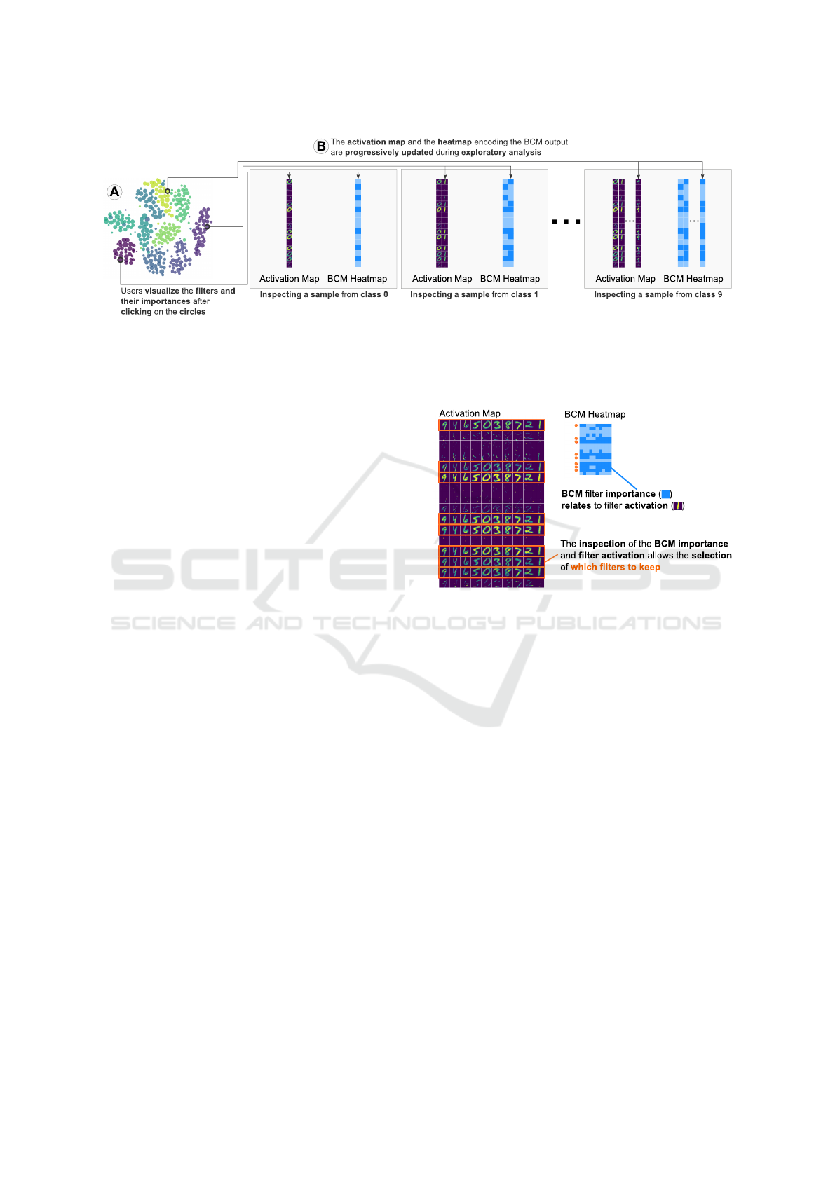
Figure 4: Assessing feature importance using Bayesian Case Model (BCM) and visualization techniques. The projection of
the test set can be seen by the scatter plot visualization in (a) to help users make sense of the similarity among data points.
After clicking on a circle of the projection, all of the activation filters are shown in another view, as seen in (b). The important
filters highlighted by BCM are encoded as a heatmap, where each cell encodes a filter, and darker blue encodes the filters
defined as important.
five (6 and 5). With such an idea in mind, it could
be interesting to verify if all the filters of a given con-
volutional layer contribute to the classification of the
hand-written digits. In this case, users would know if
their architecture needs to be more complex—when
all the filters contribute to the prediction, but the loss
is high—or if its architecture could be pruned—when
the model is already showing good performance.
We already know that our architecture is perform-
ing quite well on the MNIST dataset. Our method-
ology could be applied to find candidates to reduce
the number of parameters while maintaining as much
of the model’s performance as possible. After com-
puting the BCM for each l
2
(X
test
i
) of the test set—
that is, for each set of filter activations for all data
observations in the test set—we selected the filters
highlighted in orange of Fig. 5 as the important ones,
that is, the remaining of the filters were removed from
the Convolutional Layer II. Then, predicting the test
set with the pruned architecture resulted in 0.9278 of
accuracy and 0.247421 of loss. Here, removing the
filters that were not doing a valuable job to help the
model discriminate hand-written digits increased the
accuracy and reduced the loss. Such a result could
be explained by the fact that the filters with no useful
contribution may introduce artifacts that can confuse
the model when predicting the class of the digits with
a complex trait so that removing these filters from the
network could reduce the probability of such errors.
One may notice in Fig. 5 that a few filters seem
to present very similar activation patterns. When de-
signing a CNN, each filter of a convolutional layer is
meant to capture a different characteristic of the input
data, such as information about borders, textures, and
shape. So, if two or more filters present similar acti-
vations, it means they are redundant. The redundancy
has the same problem with filters that do not activate
Figure 5: Highlighting important filters based on the im-
portance returned by BCM (BCM heatmap) and the visual
inspection of the activations in the Activation Map.
at all, and they do not add information that the follow-
ing layers could use to discriminate among digits. As
a result, redundant filters can also be removed from
the convolutional layer.
Fig. 6 shows the features kept in the final configu-
ration of Convolutional Layer II with redundancy re-
moval in mind. In this case, by visualizing the feature
activations classified as important by the BCM tech-
nique, consecutive filters that express similar activa-
tion were removed together with the features express-
ing no contribution. After predicting the test set with
the filter configuration of Fig. 6 the model achieved
0.9281 of accuracy and 0.24984 of loss.
Although we had only a slight gain in the per-
formance after filter pruning, augmenting the perfor-
mance of deep learning models is a difficult task when
the model is already presenting good results (Rauber
et al., 2017). Moreover, removing filters means re-
moving computational operations, which leads to a
decrease in time execution to train and prediction—
a big challenge for deep learning models. Lastly,
by successively using our methodology, practitioners
Semi-automatic CNN Architectural Pruning using the Bayesian Case Model and Dimensionality Reduction Visualization
207
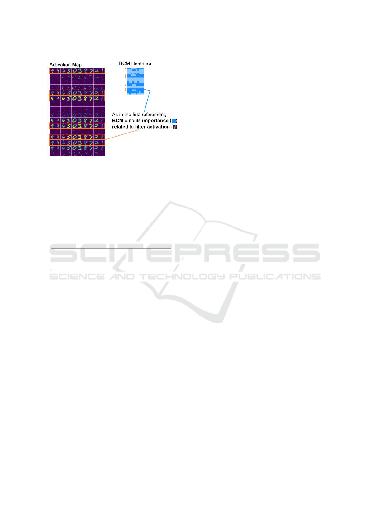
Figure 6: Using visual inspection to remove redundancy
among convolutional filters. Besides identifying useful
filters, our approach allows users to discover redundancy
among filters visually—redundant filters contribute simi-
larly and can be removed from the convolutional layer.
could build an intuition on designing more efficient
deep learning models. The performance of CNN be-
fore and after the two refinements is shown in Table 1.
Table 1: Performance of the CNN before and after two re-
finements.
Model Loss Accuracy
Initial 0.25794 0.9243
After refinement #1 0.24742 ↓ 0.9278 ↑
After refinement #2 0.24984 ↑ 0.9281 ↑
6 DISCUSSION
We demonstrated the usefulness of our approach dur-
ing the experimentation section to aid in the architec-
tural tuning of a convolutional neural network. By
employing scatterplot and heatmap visual metaphors
to emphasize the similarity among data points and the
importance of the filters, users can get an overview
of how filters react with inputs presenting higher or
lower similarity. Such a task is further improved by
the coordination mechanism that draws columns of
filter activations and filter importance as users click
on data points of interest. In this case, given two or
more data points, users can quickly inspect if filters
contribute in a contrastive fashion, contribute equally,
or even if filters do not contribute at all to the model’s
prediction.
Another interesting application of our approach
consists of allowing users to investigate the filters for
a particular cluster of images, supported by the co-
ordination between the scatterplot and the activation
map. Focusing on a group of interest, users may un-
derstand the activation patterns and how the convolu-
tional neural work made the decisions to the classifi-
cation.
One limitation of our methodology is related to
the computational complexity of the Bayesian Case
Model and by the fact that a matrix must be gener-
ated for each input image, as explained in Section 4.
Although this problem can be reduced using repre-
sentative data points of the dataset used in this work,
we plan to investigate alternative solutions further or
develop simpler versions.
Another limitation of our approach is related to
an well-known problem of representing classes us-
ing color. While humans can differentiate well ten
classes represented by colors (Ware, 2012), real-
world datasets commonly have more classes. Thus, in
order to prune deep learning models trained on more
than ten classes, the interaction mechanism to visual-
ize the filters’ patterns using the heatmap would need
a different approach, such as selection boxes on the
interface.
7 CONCLUSIONS
The design of deep learning architectures can be a te-
dious task. The most common approach is to define
models that are way too complex for the problem in
consideration and then fine-tune the architectures by
removing filters or layers. Then, the models are re-
trained with tuned architecture to achieve similar per-
formance.
In this work, we propose a semi-automatic ap-
proach that uses the Bayesian Case Model (BCM) to
identify the most important filters of convolutional
layers based on the activation of the filters. Users
can explore the dataset through scatterplot visualiza-
tion while investigating the filters’ activations and
their corresponding importance to the model’s pre-
diction using coordination mechanisms. A prelimi-
nary use case shows that BCM can select the filters
that truly contribute to the model’s performance. At
the same time, the visualization emphasizes other as-
pects that contribute to the classification performance
of datasets, such as redundancy among filters. Af-
ter removing non-important filters, the prediction with
finer CNN architectures yielded better results.
In future works, we plan to analyze more complex
datasets and well-known CNN architectures to fully
understand how much of these architectures could
be removed while maintaining performance. Besides
that, we plan to implement an entire pipeline where all
the techniques involved in our methodology would be
integrated.
IVAPP 2022 - 13th International Conference on Information Visualization Theory and Applications
208

ACKNOWLEDGEMENTS
This study was financed in part by the Coordenac¸
˜
ao
de Aperfeic¸oamento de Pessoal de N
´
ıvel Superior
- Brasil (CAPES) and by Fundac¸
˜
ao de Amparo
`
a
Pesquisa (FAPESP) [grant numbers #2018/17881-3,
#2018/25755-8].
REFERENCES
Clavien, G., Alberti, M., Pondenkandath, V., Ingold, R., and
Liwicki, M. (2019). Dnnviz: Training evolution visu-
alization for deep neural network. In 2019 6th Swiss
Conference on Data Science (SDS), pages 19–24.
Dubey, A., Chatterjee, M., and Ahuja, N. (2018). Coreset-
based neural network compression.
Garcia, R., Falc
˜
ao, A. X., Telea, A. C., da Silva, B. C.,
Tørresen, J., and Dihl Comba, J. L. (2019). A method-
ology for neural network architectural tuning using ac-
tivation occurrence maps. In 2019 International Joint
Conference on Neural Networks (IJCNN), pages 1–10.
Goodfellow, I., Bengio, Y., and Courville, A. (2016). Deep
Learning. MIT Press.
He, Y., Liu, P., Wang, Z., Hu, Z., and Yang, Y. (2019). Filter
pruning via geometric median for deep convolutional
neural networks acceleration.
He, Y., Zhang, X., and Sun, J. (2017). Channel pruning for
accelerating very deep neural networks.
Hofmann, T. (1999). Probabilistic latent semantic index-
ing. In Proceedings of the 22Nd Annual International
ACM SIGIR Conference on Research and Develop-
ment in Information Retrieval, SIGIR ’99, pages 50–
57, New York, NY, USA. ACM.
Hohman, F., Park, H., Robinson, C., and Polo Chau, D. H.
(2020). Summit: Scaling deep learning interpretabil-
ity by visualizing activation and attribution summa-
rizations. IEEE Transactions on Visualization and
Computer Graphics, 26(1):1096–1106.
Kim, B., Rudin, C., and Shah, J. (2014). The bayesian case
model: A generative approach for case-based reason-
ing and prototype classification. In Proceedings of the
27th International Conference on Neural Information
Processing Systems - Volume 2, NIPS’14, pages 1952–
1960, Cambridge, MA, USA. MIT Press.
LeCun, Y. and Cortes, C. (2010). MNIST handwritten digit
database.
Li, G., Wang, J., Shen, H.-W., Chen, K., Shan, G., and Lu,
Z. (2021). Cnnpruner: Pruning convolutional neural
networks with visual analytics. IEEE Transactions on
Visualization and Computer Graphics, 27(2):1364–
1373.
Liu, S., Maljovec, D., Wang, B., Bremer, P., and Pascucci,
V. (2017a). Visualizing high-dimensional data: Ad-
vances in the past decade. IEEE Trans. Vis. Comput.
Graph., 23(3):1249–1268.
Liu, Z., Li, J., Shen, Z., Huang, G., Yan, S., and Zhang,
C. (2017b). Learning efficient convolutional networks
through network slimming.
Luo, J.-H., Wu, J., and Lin, W. (2017). Thinet: A filter level
pruning method for deep neural network compression.
Marcilio-Jr, W. E., E. D. M. (2020). Sadire: a context-
preserving sampling technique for dimensionality re-
duction visualizations. J Vis, 23:999–1013.
Marcilio-Jr, W. E., Eler, D. M., Garcia, R. E., Correia, R.
C. M., and Silva, L. F. (2020). A hybrid visualiza-
tion approach to perform analysis of feature spaces.
In Latifi, S., editor, 17th International Conference
on Information Technology–New Generations (ITNG
2020), pages 241–247, Cham. Springer International
Publishing.
Marc
´
ılio-Jr, W. E., Eler, D. M., Paulovich, F. V., and Mar-
tins, R. M. (2021a). Humap: Hierarchical uniform
manifold approximation and projection.
Marc
´
ılio-Jr, W. E., Eler, D. M., Paulovich, F. V., Rodrigues-
Jr, J. F., and Artero, A. O. (2021b). Explorertree: A fo-
cus+context exploration approach for 2d embeddings.
Big Data Research, 25:100239.
Pezzotti, N., H
¨
ollt, T., Van Gemert, J., Lelieveldt, B. P. F.,
Eisemann, E., and Vilanova, A. (2018). Deepeyes:
Progressive visual analytics for designing deep neu-
ral networks. IEEE Transactions on Visualization and
Computer Graphics, 24(1):98–108.
Rauber, P. E., Fadel, S. G., Falc
˜
ao, A. X., and Telea, A. C.
(2017). Visualizing the hidden activity of artificial
neural networks. IEEE Transactions on Visualization
and Computer Graphics, 23(1):101–110.
Reingold, E. M. and Tilford, J. S. (1981). Tidier drawings
of trees. IEEE Transactions on Software Engineering,
SE-7(2):223–228.
Strobelt, H., Gehrmann, S., Pfister, H., and Rush, A. M.
(2018). Lstmvis: A tool for visual analysis of hidden
state dynamics in recurrent neural networks. IEEE
Transactions on Visualization and Computer Graph-
ics, 24(1):667–676.
Ware, C. (2012). Information Visualization: Perception for
Design. Morgan Kaufmann Series in Interactive Tech-
nologies. Morgan Kaufmann, Amsterdam, 3 edition.
Yu, R., Li, A., Chen, C.-F., Lai, J.-H., Morariu, V. I., Han,
X., Gao, M., Lin, C.-Y., and Davis, L. S. (2018).
Nisp: Pruning networks using neuron importance
score propagation.
Zeiler, M. D. and Fergus, R. (2014). Visualizing and under-
standing convolutional networks. In Fleet, D., Pajdla,
T., Schiele, B., and Tuytelaars, T., editors, Computer
Vision – ECCV 2014, pages 818–833, Cham. Springer
International Publishing.
Semi-automatic CNN Architectural Pruning using the Bayesian Case Model and Dimensionality Reduction Visualization
209
