Accelerated Variant of Reinforcement Learning Algorithms for Light

Control with Non-stationary User Behaviour

Nassim Haddam

, Benjamin Cohen Boulakia

and Dominique Barth

LINEACT - Recherche & Innovation, CESI, Nanterre, France

DAVID Laboratory, Paris-Saclay - UVSQ, Versailles, France

Keywords:

Smart Building, Reinforcement Learning, Light Control, Light Comfort.

Abstract:

In the context of smart building energy management, we address in this work the problem of controlling

light so as to minimise energy usage of the building while maintaining the satisfaction of the user regarding

comfort using a stateless Reinforcement Learning approach. We consider that the user can freely interact with

the building and changes the intensity of the light according to his comfort. Moreover, we consider that the

behaviour of the user depends not only on present conditions but also on past behaviour of the control system.

In this setting, we use the pursuit algorithm to control the signal and investigate the impact of the discretization

of the action space on the convergence speed of the algorithm and the quality of the policies learned by the

agent. We propose ways to accelerate convergence speed by varying the maximal duration of the actions while

maintaining the quality of the policies and compare different solutions to achieve it.

1 INTRODUCTION

Energy consumption in buildings forms a large part

of energy consumption world-wide. Indeed, global

buildings account for 30% of total energy in 2019

(GABC, 2020). Energy cost is used to satisfy hu-

man needs, but it is expected that a big part of it can

be saved if resources are managed intelligently. Re-

cent technological advances to capture, store and pro-

cess data have developed at an increasing rate. More

precisely, one of the questions treated by the research

community is to conceive control systems which are

capable of learning human preferences and to deter-

mine which actions to take in order to reduce energy

costs and satisfy human needs.

Related Work: This question has attracted a lot of

attention in the recent years, be it on thermal con-

trol (et al, 2012) (et al, 2018) (Yang et al., 2015), or

light control (Cheng et al., 2016) (Park et al., 2019),

(Zhang et al., 2021).

In light control, most of the methods used are

based on distributions which are extracted from in-

teraction of the user with the building. The ﬁrst sys-

tems which were used were equipped of PIR sen-

sors and did simply switch on/off the lights according

to room occupacy (Neida et al., 2001), (F.Reinhart,

2004), (Jennings et al., 2000). But those approaches

wasted energy due to Time Delays in sensors activa-

tion (Nagy et al., 2015). In (Garg and N.K.Bansal,

2000), a statistical method based on frequency of

Time Delays to model the occupant’s activities is pro-

posed. The Time Delay is adapted to each occupant

and achieved energy saving close to 5%. The work

on (Nagy et al., 2015) was inspired by (Garg and

N.K.Bansal, 2000) to include illuminance levels in

the model. We argue that these methods are limited

in that they do not directly optimize energy usage.

A more direct way to control lighting is to opti-

mize energy use by controlling the signal (which rep-

resents the light intensity) so as to optimize an ob-

jective function. This approach requires the model to

have knowledge about user preferences. One way of

doing so is by means of a model of user behavior. Sev-

eral models have been proposed to model user com-

fort in terms of visual comfort (Mardaljevic, 2013),

(P. Petherbridge, 1950), (Einhorn, 1979) but the ma-

jority of those models presuppose that we know cer-

tain elements of the environment which aren’t readily

available. The models might need for instance the in-

clination of the head, the number of glare in the visual

ﬁeld of the user, the distance to lights sources...etc.

Our Contribution: An alternative to this approach

is to use Reinforcement Learning (RL). Contrary to

thermal comfort, there is very little work done to

control signal value using Reinforcement Learning

(Cheng et al., 2016), (Park et al., 2019). Reinforce-

ment Learning is a really ﬂexible framework and al-

lows the system to learn optimal control policies (with

Haddam, N., Boulakia, B. and Barth, D.

Accelerated Variant of Reinforcement Learning Algorithms for Light Control with Non-stationary User Behaviour.

DOI: 10.5220/0010987900003203

In Proceedings of the 11th International Conference on Smart Cities and Green ICT Systems (SMARTGREENS 2022), pages 78-85

ISBN: 978-989-758-572-2; ISSN: 2184-4968

or without a model), some behaviour speciﬁed by the

optimization of a reward signal coming from the en-

vironment. In the present work, we study more effec-

tive variants of the algorithm proposed on (Haddam

et al., 2020) and propose ways to accelerate conver-

gence. The same user model was used, special care

were given to its parameters and their relation to the

performances of the algorithms, especially the sensi-

bility of the user and its memory.

Provided that we are in a setting where the user

has memory of the history of the signal, where low

signal values are a source of discomfort for the user,

and where we reduce energy by reducing signal value,

the contributions of the present paper are as follows.

In section 3 we compare the performances of different

stateless Reinforcement Learning algorithms which

are presented in section 2. We also provide detailed

insight on the performance of the LRI algorithm (as

proposed on (Haddam et al., 2020)) and the pursuit

algorithm, which is generally faster on stationary en-

vironments. In section 4, we study the performances

of the pursuit algorithm for different set of actions of

the action space. We also propose ways to improve

speed and quality of convergence of the proposed al-

gorithm. Finally, in section 5 we present some ﬁnal

remarks and perspectives regarding our work.

2 CONTROL WITH RL

In this section, we present how to model our problem

using Reinforcement Learning. We start by introduc-

ing some notations in order to deﬁne the actions of

the agent. We then proceed to deﬁne how the policy

is represented in our problem. Finally, we present the

Reinforcement Learning algorithms we studied. We

emphasize that the goal here is not to learn or guess

the user’s model, even if we use a user model for sim-

ulation purposes as modeled in (Haddam et al., 2020).

We consider that the actions available to the agent

are a bunch of speeds of light signal decrease. Those

are the slopes the signal takes during its decrease. We

deﬁne the set of actions AC = {sl ∈ R

−

∗

| sl

max

≤ sl ≤

min

} where sl

min

and sl

max

are the smoothest and

steepest slopes available to the agent. The control sys-

tem selects a slope sl and then proceeds to apply the

selected control strategy time step by time by lower-

ing the signal according to the selected slope. The

maximal duration of an action noted max dur is set

before the control starts. Upon applying a slope, if

the user intervenes, or if the user does not intervene

during max dur time steps, the action chosen by the

agent is stopped and the agent updates its policy as to

chose good control strategies more often.

We propose multiple ways to set the maximal du-

ration of the actions. The ﬁrst way is obviously to

impose an inﬁnite maximal duration. In this case, the

system has no say on how long an action might take,

and only the interventions of the user matter. The sec-

ond way is to impose a ﬁxed duration limit. In this

case, the maximal duration of all the actions is the

same and doesn’t change with time (we call it a static

maximal duration). The third way is to change the

maximal duration with time. This case is named dy-

namic maximal duration. For this case, the maximal

duration is the same for all actions, but changes de-

pending on past behaviour of the user. The idea is

that the current action could be deactivated to choose

another one if the user takes much longer to intervene

than usual. We propose two update rules for dynamic

maximal duration.

We consider the intervention time of an action to

be the time between the moment where the action is

chosen and the moment where the user intervenes.

The update rules of dynamic maximal duration de-

pend both on the average and the standard deviation

of the intervention time. In this case, the action to be

taken could be chosen again if the duration of the cur-

rent action exceeds the average duration of the user’s

intervention by a factor of the standard deviation of

the intervention time (time of the current action >av-

erage intervention time + const × standard deviation

of the intervention time). The ﬁrst update rule for the

dynamic maximal duration is to set it as the sum of

the average of the intervention time and a factor of

the standard deviation of the intervention time (we

name it update mean var interv). The second update

rule is the same as the ﬁrst update rule by assuming

that the law of probability of the intervention time of

the user is an Exponential probability law (even if the

memory-less assumption of the Exponential distribu-

tion doesn’t hold in the context of a non-stationary

user). The last update rule gives a way to approx-

imate the standard deviation and alleviates the need

to memorize past intervention times and thus might,

at least, reduces computation time. For this rule, the

standard deviation is therefore the root square of the

mean, and we call it update mean interv.

As stated previously, we use learning algorithms

using the framework of Reinforcement Learning (RL)

(Sutton and Barto, 1998). The policy of the agent is

represented using a stochastic vector. The vector is

updated each time the action ﬁnishes, and is thus de-

ﬁned for each k-th user intervention. The policy of

the agent following the k-th user intervention is rep-

resented by the stochastic vector p

∈ [0, 1]

|SL|

where

[i] is the probability of choosing the i-th least steep

slope of SL.

Accelerated Variant of Reinforcement Learning Algorithms for Light Control with Non-stationary User Behaviour

The reward of an action applied by the agent from

time step n to time step n

is decomposed in two parts:

a part reﬂecting energy consumption noted ren

n,n

and

a part reﬂecting user comfort noted rcs

n,n

. Together,

those two parts form the complete reward which is

n,n

= ren

n,n

.rcs

n,n

where γ is a strictly positive real

number. The parameter γ represents how strongly we

reward the control system for satisfying the user. De-

tails concerning the reward are on (Haddam et al.,

2020).

2.1 The Learning Algorithms

The learning algorithms which were selected for our

work are represented as RL agents where the al-

gorithm used for learning is LRI (Linear Reward

Inaction) (Thathachar, 1990), LRP (Linear Reward

Penalty) (Thathachar, 1990), and the pursuit algo-

rithm (Kanagasabai et al., 1996). The remainder of

this section presents the LRI algorithm, the LRP and

the pursuit algorithm.

In the LRI algorithm, the policy is represented as

a stochastic vector and is updated as to increase the

probability of the action selected by the agent linearly

to its reward. Suppose a strategy sl has triggered the

k-th intervention of the user. Suppose sl has index

i[sl] in vector (policy) p

. Then, according to LRI, p

is updated for each k as follows

k+1

:= p

+ α.r

n,n

.(e

i[sl]

− p

) (1)

where e

i[sl]

is the unitary vector of unit value in the

component associated with the slope sl in p

. An-

other variant of LRI which is called the LRP (Lin-

ear Reward Penalty) decreases the probability of the

actions which didn’t lead to any reward (in addition

to increasing the probability of the actions leading to

good reward like LRI).

The idea of the pursuit algorithm is to reinforce

not the action chosen at the current moment, but the

action that has the best estimate among the available

actions. To this end, the algorithm will have to keep

in memory the estimates constructed from the rewards

obtained by each action. The probability of the action

which has the best estimate is increased linearly. If

we pick the same notations as before, we can sum-

marize the operations of the pursuit algorithm by the

formulas which follows. The update of the policy in

the pursuit algorithm is

k+1

:= p

+ α.(e

− p

) (2)

where h is the index of the best action according to

the estimate of the algorithm.

3 COMPARING RL

ALGORITHMS

In this section, we start by comparing the pursuit al-

gorithm and the LRI algorithm (in terms of speed and

quality of convergence) for a typical setting we con-

sidered to get a visual feel for the behaviour of the

algorithms. We then do a more systematic compari-

son of the LRI, the LRP and the pursuit algorithms to

provide quantitative estimation of the speed of con-

vergence independently of the parameters of the sim-

ulation. This comparison allows us to select the most

appropriate algorithm for our problem.

3.1 The Pursuit Algorithm

The experiment we do here extends on (Haddam et al.,

2020) done on the LRI algorithm. We run the pur-

suit algorithm and the LRI 30 times for 1000000

time steps with the user with medium-term memory

(the value of the present effect parameter pe is set

to pe = 0.35). We select the user with medium-term

memory (pe = 0.35) to not draw conclusions on ex-

treme cases (memory which is too small or too large).

In order to observe the behaviour of the algorithm, the

learning rate is ﬁxed to 0.001. The value of the learn-

ing rate was chosen as low as possible to allow the

algorithm to converge at a reasonable time. All the

estimates are initialized to 0 for the pursuit algorithm

(a classical choice which is relevant here because the

agent is pessimistic in that all the slopes are bad). The

reward is monitored during the run. We take the mean

of the reward over the executions. The results are de-

picted on the curves (Figure 1) containing the mean

values. The stochastic vectors at the end of each run

are outlined in Figure 1.

We note from the curves that the pursuit algo-

rithm converges a lot faster than the LRI algorithm

(nearly 10 times faster). The policies learned by the

pursuit algorithm are also of better quality, as the al-

gorithm converges nearly every time. As the pur-

suit algorithm estimates directly the reward of the ac-

tions, it may form a better way to deal with the ex-

ploration vs exploitation dilemma characterizing Re-

inforcement Learning problems, because as the agent

gains knowledge from the environment, the action es-

timated to be the best changes less and less frequently,

and the stochastic vector converges more rapidly to it.

But because only the probability of the best ac-

tion according to the agent is updated, the agent may

also be tempted to exploit the learned actions more

than necessary. Furthermore, the case of study con-

sidered in this paper is such as the environment is

non-stationary because its state changes in response to

SMARTGREENS 2022 - 11th International Conference on Smart Cities and Green ICT Systems

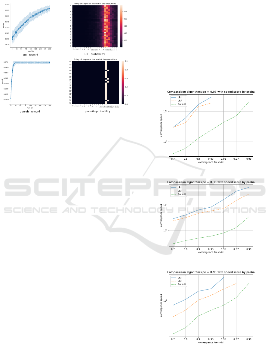
Figure 1: The LRI vs. the pursuit algorithm - 1000000 time

steps. For the left column, the x-axis is the time, the y-axis

is the reward. For the right column, the x-axis is the index

of the slope, the y-axis is the execution number.

the agent, which differs sensibly from the cases most

commonly studied by researchers. For those reasons,

we present in the next subsection a more quantitative

comparison between various Reinforcement Learning

algorithms.

3.2 Comparison of RL Algorithms

In this section, we compare different (stateless) Re-

inforcement Learning algorithms to identify the algo-

rithms most suitable for our problem. We took differ-

ent parameters of the algorithm and the user. The al-

gorithms are tested during 3000000 time steps (subdi-

vided as before into intervals of size 5000 time steps)

for 30 runs for different hyperparameters set. The al-

gorithms are then compared by taking the best hyper-

parameter for each one. A criterion for quality of con-

vergence and speed of convergence were chosen to

account effectively for the comparison. For each algo-

rithm, the best hyperparameter is chosen by ﬁrst tak-

ing only those for which the algorithm is considered

to be convergent (i.e. when the empirical stochastic

vector has a predeﬁned fraction of its weight concen-

trated on the best action and one of its left or right

neighbors). After ﬁltering the bad values of the hyper-

parameters by the convergence criteria, the best value

is chosen by then taking the value of the hyperpa-

rameters which has achieved convergence the fastest

(using the same threshold as the ﬁrst step). This se-

lection process was applied for different convergence

thresholds (for the values 0.7, 0.8, 0.9, 0.93, 0.95,

0.97, 0.99) each time taking the best hyperparame-

ters and the results are shown in Figure 2. Figure

2 shows a comparison on the speed of convergence

of the above-mentioned algorithms for the values of

pe considered earlier (long term user for pe = 0.05,

medium term user for pe = 0.35, and short term user

for pe = 0.95 from top to bottom). The abscissa axis

represents the convergence thresholds, and the ordi-

nate axis represents the number of intervals required

for each algorithm to converge at the corresponding

threshold. The values on the y-axis are displayed on

logscale for good visualization. Algorithms which

didn’t converge for any of the tested values of the hy-

perparameters were not included on the ﬁgure.

(a) Comparison with pe = 0.05.

(b) Comparison with pe = 0.35.

Figure 2: Comparison of the speed of convergence for the

algorithms : LRI, LRP, the pursuit and the hierarchical pur-

suit.

Accelerated Variant of Reinforcement Learning Algorithms for Light Control with Non-stationary User Behaviour

We note that there are roughly two kinds of algo-

rithms in terms of speed of convergence, those which

takes really long to converge or don’t converge at all

for all types of users (LRI, LRP) and the ones which

converges very well on all kinds of users (pursuit).

In terms of the memory of the user and its relation

with convergence speed, we notice that the case of a

medium-term memory user (pe = 0.35) seems to be

the easiest one for all the algorithms considered. The

short-term memory user (pe = 0.95) is challenging

for the algorithms, probably because the user changes

abruptly if the next action is too different from the

current action (especially for steep slopes). The case

of a long-term memory user (pe = 0.05) is also hard

because the reactions of the user depend on control

far in the past so that the behaviour of the user might

change too much for the same action depending on

past actions chosen by the system. In the following,

we present a discussion on the performances of the

three algorithms.

The LRI and LRP algorithms converge very

slowly (50 to 110 bins). Concerning the LRI algo-

rithm, the most common reason for slow convergence

is that the learning rate has to be set low so that the

agent won’t be stuck on suboptimal action. For the

LRP algorithm, however, which decreases the proba-

bilities of actions not leading to a good outcome. The

slow convergence rate might be better explained by

the fact that the stochastic vector juggles around too

often before leading to good actions.

According to our experiment, the pursuit algo-

rithm seems to be the fastest algorithm (an order

of magnitude faster than LRI and LRP). The update

strategy of the pursuit algorithm and its variants might

form a better way to balance effectively between ex-

ploration and exploitation than LRI. In fact, the best

estimated action changes less and less as the algo-

rithm gains knowledge about its environment. This

could make the pursuit algorithm more stable than

LRI and LRP and allows us to set higher learning rates

for the algorithm without suffering performance loss

as with the LRI algorithm. We can conclude from our

experiment that the pursuit algorithm is the most ade-

quate for our problem, independently of the memory

of the user and the learning rate.

4 ACCELERATION OF THE

ALGORITHMS

We propose in this section ways to accelerate the pur-

suit algorithm which was selected by the preceding

experiments. The ﬁrst approach to greatly enhance

the speed of convergence of the algorithm is to vary

the maximal duration of the actions (discretization of

the time). The second way to speed up the algorithm

is to determine the best set of actions available to the

agent (discretization of the action space). We also

show how the set of actions available to the agent

greatly inﬂuences the speed of convergence of the al-

gorithm.

4.1 Maximal Duration of the Actions

To speed up the convergence of Reinforcement Learn-

ing algorithms in our problem, we propose to dy-

namically change the maximal duration of the actions

while learning. The following experiment shows the

effect of changing the maximal duration of the action

on the speed of learning. The number of executions

is 30 and the number of time steps per execution is

1,500,000. The time is subdivided into sub-intervals

of size 5000 from which we take only the mean of

the values calculated (the reward, the energy, and the

value of the sensibility of the user m). The learn-

ing rate is ﬁxed at 0.002. The experiment was done

for different values of the present effect parameter,

namely 0.05, 0.35 and 0.95.

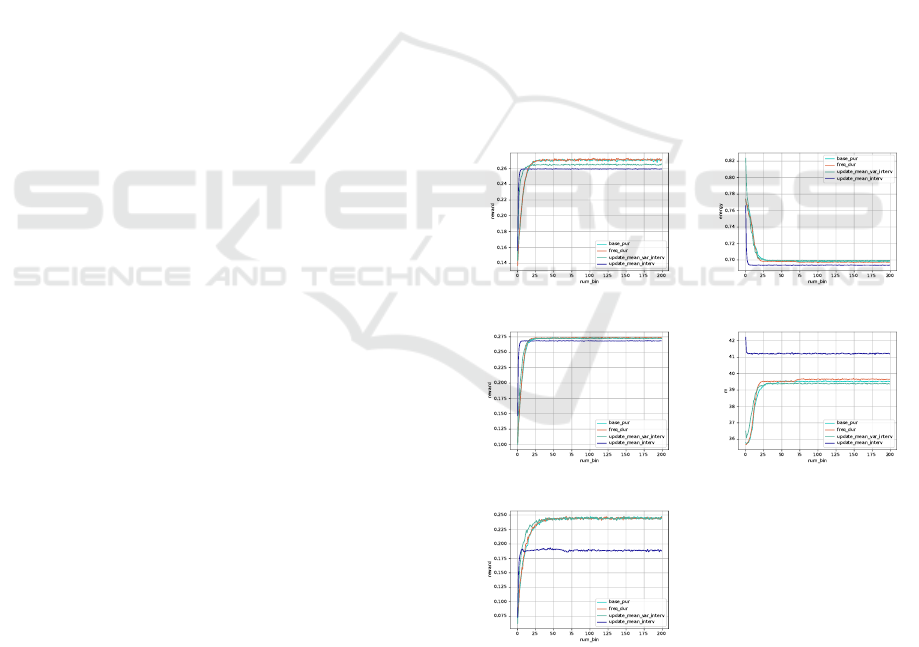
pe = 0.05 - reward pe = 0.35 - energy

pe = 0.35 - reward pe = 0.35 - m

pe = 0.95 - reward

Figure 3: Comparison of the performances of the algorithm

between different ways to set the decision type and differ-

ent sizes of the memory of the user, long-term (pe = 0.05),

medium term (pe = 0.35) and short-term (pe = 0.95).

The graphs (on Figure 3) show the performance

of the control system with the pursuit algorithm for

SMARTGREENS 2022 - 11th International Conference on Smart Cities and Green ICT Systems

Figure 4: Heatmaps of the stochastic vectors at the end

of each run whe pe = 0.35. (a), (b), (c) and (d) are the

cases base pur, freq dur, update mean var interv and up-

date mean interv respectively.

the case where the decision is made at each user in-

tervention (named base pur), set to a ﬁxed maximal

duration (named freq dur). The graphs depict also

the performances of the system with the two ways

to use the update rule of the dynamic maximal du-

ration of the actions. The ﬁrst one corresponding to

update mean var interv), and the second case corre-

sponding to update mean interv). The left column

of Figure 3 shows from top to bottom the evolution

through time of the reward for the case where pe =

0.35. The right column shows the evolution through

time of the value of energy and the value of m. For

the curves where the maximal duration of an action

is ﬁxed, those durations were the best value among

the values {1, 5, 10, 25, 50, 100} for each value of pe.

For the cases where the maximal duration of the ac-

tions changes, the factor associated to the standard de-

viation is also chosen to be the best value amongst

{1, 2, 3, 4} for each pe. We also display the heatmaps

(Figure 4 for the case pe = 0.35) of the stochastic vec-

tors at the end of training. On the heatmaps, the axes

are labelled by the indices of the slopes (x-axis) and

by the run (y-axis).

From the curves, we can observe that the re-

ward stabilizes the fastest where the update rule

for the maximal duration of the actions is up-

date mean interv for all values of pe. Further-

more, the case update mean var interv also stabilizes

rapidly for the case where we have a long-term mem-

ory user and a short-term memory user (pe = 0.05

and pe = 0.95) and is even a little higher at the be-

ginning of training for the case of a medium-term

memory user (pe = 0.35). The aforementioned obser-

vations show the pertinence of using dynamic maxi-

mal duration of the actions, especially as the conver-

gence speed is better than the case where the decision

time is set to a maximal limit (the cases base pur and

freq dur).

One of the drawbacks of dynamic maximal dura-

tion is that the high convergence speed comes at the

cost of a low reward at the end (especially for the shot-

term memory user, where the state of the user depends

mostly on the present). This can be explained by the

fact that the principle of dynamic maximal duration

of the actions is to stop the slopes (mostly soft slopes

because they are the slowest) before the user inter-

venes, which means that steep slopes will be played

a little more often. The playing of steep slopes trig-

gers more reactions from the user (probably the most

frequently when the user has short memory). But this

phenomenon is a rather mild hindrance because the

user is kept at a state close to its most favorable state

(m = 41 at worst knowing that m

= 35, it is 10% of

the maximal possible value for m) and the energy used

to do so is lesser for the dynamic maximal duration

of the actions rules. Only the case where pe = 0.35

is shown, but the conclusions hold even for the other

cases (pe = 0.05, pe = 0.95). We can also see from

the heat maps associated to the medium-memory user

that the algorithm converges close to the best slope

(slope 17) when dynamic maximal duration of the ac-

tions is used (in fact, they converge even for other val-

ues of pe which are not shown here to not clutter up

the reading of the article).

Another relatively mild drawback of the dynamic

maximal duration of the actions is convergence to ex-

actly the optimal action, we observe that the base case

converges more often to the optimal action than the

dynamic maximal duration of the actions cases. We

can, therefore, conclude that controlling the maximal

duration of the actions allows increasing greatly the

speed of convergence of the algorithm.

4.2 Effect of the Number of Actions on

Learning

In this subsection, we study the inﬂuence of the num-

ber of actions on the speed of convergence of the al-

gorithm. The experience we present in this subsection

consists in launching for 30 times the control system

for different sets of actions (slopes) corresponding to

different action spaces. Those sets correspond to the

slopes where the gap between two successive slopes

is 5, 10, 15 and 20. Before doing the experiment,

the best slope was calculated for each set of actions

and for each value of pe by repeating them and cal-

culating the mean reward, the mean energy, and the

Accelerated Variant of Reinforcement Learning Algorithms for Light Control with Non-stationary User Behaviour

mean value of m during the runs. We note that the

optimal action in terms of the reward is the same for

the set of actions associated with gaps 5 and 15. The

set of actions associated with gaps 10 and 20 have

different optimal actions. The algorithm used is the

pursuit algorithm, where the learning rate is set to the

value lr = 0.001. Each execution has a duration of

1500000 time steps decomposed into intervals of size

5000 where the mean value of the energy, the reward

and the value of m are observed. We also calculate

the mean of those values for all the executions. The

results are shown on Figure 5 for each value of pe

(0.05, 0.35, 0.95).

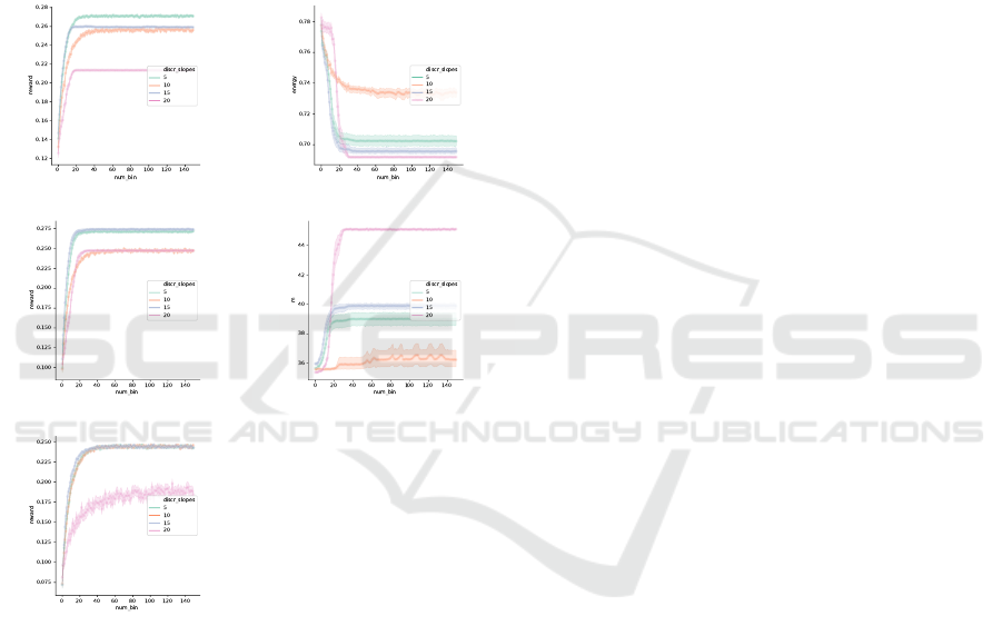
pe = 0.05 - reward pe = 0.35 - energy

pe = 0.35 - reward pe = 0.35 - m

pe = 0.95 - reward

Figure 5: The evolution of the reward (left), the energy (top

right), and the state of the user (center right) for the set of

actions of gaps 5, 10, 15 and 20 for the slopes.

Each row corresponds to the result of the experi-

ment for different values of pe (0.05, 0.35, 0.95). The

left column corresponds to the evolution over time of

the reward for all the values of pe. The right column

corresponds to the evolution over time of the energy

and the value of m for pe = 0.35. We ﬁrst note that

the system improves over time for all the metrics apart

from the user state (but the user still remains at the ac-

ceptable range because the value of the m parameter

is close to the lowest value m

= 35 for all cases).

The second observation we make is that the perfor-

mances of the system do not vary linearly with the set

of actions (this seems to hold for each value of pe)

especially when pe is small. In fact, for the long-term

memory user it is clear that the best set of actions in

terms of speed of convergence are in descending order

5, 15, 10, 20.

Second, let us analyze the medium-term memory

user. We note that the best set of actions is obtained

when the gap between actions is 15 and the perfor-

mances drop the further we go from this set of actions

both in terms of speed of convergence and quantity of

reward achieved by the agent. With the set of actions

where the gap is 20, we note very low energy usage.

On the other hand, the user appears to be in a bad state

relatively to the other cases because the value of m ap-

proaches 45 (half of the signal value interval). The set

of actions associated with the gap value 10 achieves

the same reward as the previous one, but we can see

that energy usage is way higher and the state of the

user is way lower than before. Another observation

we make is that even when the optimal actions are

the same for different set of actions (for example the

5 and 15 set of actions have similar optimal actions),

the behaviour of the user and the algorithm change

qualitatively.

A possible interpretation for the observations

mentioned previously is that there is a trade-off to

be taken into account in this case. If we take a very

coarse set of actions of the action space, the optimal

action (on all sets) may not be on the selected set of

actions which leads the algorithm to learn subopti-

mal actions, but if the set of actions is too dense the

system may take way longer to learn the best action

because the system needs to try all of them enough

times to identify the best action. The selected set

of actions may affect the convergence of the algo-

rithm, even when the optimal actions are the same

for different sets of actions. A possible approach to

deal with those issues is to consider using methods

which handle large action spaces by ﬁltering rapidly

the good actions from the bad ones. Hierarchical

methods (Yazidi et al., 2019) may be a good alter-

native to explore to deal with this drawback. Finally,

we can conclude that the best set of actions is where

the gap is 5 for the user with a long-term memory and

where the gap is 15 for the user with a medium-term

memory. And for a user with a short-term memory,

we also prefer to choose the set of actions associated

with gap 15 because it seems better at the beginning

of learning.

SMARTGREENS 2022 - 11th International Conference on Smart Cities and Green ICT Systems

5 CONCLUSION AND

PERSPECTIVES

In this paper, we propose ways to improve the con-

vergence of Reinforcement Learning algorithms for

light signal control to reduce energy costs while sat-

isfying the user. The setting considered in this work

is when the reactions of the user depend not only on

present conditions but on the entire history of the sig-

nal values. Furthermore, we consider the use of a sin-

gle light source and no change in the activity of the

user. We present a detailed study to determine which

Reinforcement Learning algorithm is most appropri-

ate for the problem at hand. The pursuit algorithm

seems to be the way to go for our problem.

In a future work, we consider taking into account

the global lighting environment with several light

sources where the activity of the user could vary in

the building. We also consider to look into the per-

formances of other variants of the pursuit algorithm

(like the hierarchical pursuit algorithm) and compare

its performances with other stateless Reinforcement

Learning algorithms. This comparison will allow us

to make ﬁner conclusions on the behaviour of the al-

gorithms on our problem, and possibly to circumvent

the burden of choosing the best set of actions. Also,

we consider to look into other variants of the Re-

inforcement Learning framework, particularly state-

based Reinforcement Learning. Challenges to do so

include choosing which elements might be relevant as

to determine the state and the size of the state. Other

areas of building control like HVAC control might

also beneﬁt from our work, provided we take into ac-

count inertia phenomena and more complex energy

consumption models in our approaches.

REFERENCES

Cheng, Z., Zhao, Q., Wang, F., Jiang, Y., Xia, L., and

Ding, J. (2016). Satisfaction based q-learning for in-

tegrated lighting and blind control. Energy and Build-

ings, 2016.

Einhorn, H. (1979). Discomfort glare: a formula to bridge

differences. Lighting Research and Technology.

et al, P. M. F. (2012). Neural network pmv estimation for

model-based predictive control of hvac systems. IEEE

World Congress on Computational Intelligence.

et al, S. L. (2018). Inference of thermal preference proﬁles

for personalized thermal environments. Conference:

ASHRAE Winter Conference 2018.

F.Reinhart, C. (2004). Lightswitch-2002: a model for

manual and automated control of electric lighting and

blinds. Solar Energy, 77:15–28.

GABC (2020). The global alliance for buildings and con-

struction (gabc). Technical report, The Global Al-

liance for Buildings and Construction.

Garg, V. and N.K.Bansal (2000). Smart occupancy sensors

to reduce energy consumption. Energy and Buildings,

32:91–87.

Haddam, N., Boulakia, B. C., and Barth, D. (2020). A

model-free reinforcement learning approach for the

energetic control of a building with non-stationary

user behaviour. 4th International Conference on

Smart Grid and Smart Cities, 2020.

Jennings, J. D., Rubinstein, F. M., DiBartolomeo, D., and

Blanc, S. L. (2000). Comparison of control options

in private ofﬁces in an advanced lighting controls

testbed. Journal of Illuminating Engineering Society,

29:39–60.

Kanagasabai, R., , and Sastry, P. S. (1996). Finite time anal-

ysis of the pursuit algorithm for learning automata.

IEEE Transactions on Systems, Man, and Cybernet-

ics, Part B (Cybernetics).

Mardaljevic, J. (2013). Rethinking daylighting and compli-

ance. SLL/CIBSE International Lighting Conference.

2013.

Nagy, Z., Yong, F. Y., Frei, M., and Schlueter, A. (2015).

Occupant centered lighting control for comfort and

energy efﬁcient building operation. Energy and Build-

ings, 94:100–108.

Neida, B. V., Maniccia, D., and Tweed, A. (2001). An anal-

ysis of the energy and cost savings potential of occu-

pancy sensors for commercial lighting systems. Jour-

nal of Illuminating Engineering Society, 30:111–125.

P. Petherbridge, R. H. (1950). Discomfort glare and the

lighting of buildings. Transactions of the Illuminating

Engineering Society.

Park, J. Y., Dougherty, T., Fritz, H., and Nagy, Z. (2019).

LightLearn: An adaptive and occupant centered con-

troller for lighting based on reinforcement learning.

Building and Environment.

Sutton, R. S. and Barto, A. G. (1998). Introduction to Re-

inforcement Learning. MIT Press, Cambridge, MA,

USA, 1st edition.

Thathachar, M. A. L. (1990). Stochastic automata and

learning systems. Sadhana, Vol 15, 1990.

Yang, L., Zolt

an, N., Gofﬁn, P., and Schlueter, A. (2015).

Reinforcement learning for optimal control of low ex-

ergy buildings. Applied Energy.

Yazidi, A., Zhang, X., Jiao, L., and Oommen, B. J. (2019).

The hierarchical continuous pursuit learning automa-

tion: a novel scheme for environments with large

numbers of actions. IEEE transactions on neural net-

works and learning systems, 31(2):512–526.

Zhang, T., Baasch, G., Ardakanian, O., and Evins, R.

(2021). On the joint control of multiple building sys-

tems with reinforcement learning. e-Energy ’21: Pro-

ceedings of the Twelfth ACM International Confer-

ence on Future Energy Systems, pages 60–72.

Accelerated Variant of Reinforcement Learning Algorithms for Light Control with Non-stationary User Behaviour