Survival Analysis Algorithms based on Decision Trees with Weighted

Log-rank Criteria

Iulii Vasilev

, Mikhail Petrovskiy

and Igor Mashechkin

Computer Science Department of Lomonosov Moscow State University, MSU, Vorobjovy Gory, Moscow, Russia

Keywords:

Machine Learning, Survival Analysis, Cox Proportional Hazards, Survival Decision Trees, Weighted Log-

rank Split Criteria, Bagging and Boosting Ensembles.

Abstract:

Survival Analysis is an important tool to predict time-to-event in many applications, including but not limited

to medicine, insurance, manufacturing and others. The state-of-the-art statistical approach is based on Cox

proportional hazards. Though, from a practical point of view, it has several important disadvantages, such as

strong assumptions on proportional over time hazard functions and linear relationship between time indepen-

dent covariates and the log hazard. Another technical issue is an inability to deal with missing data directly.

To overcome these disadvantages machine learning survival models based on recursive partitioning approach

have been developed recently. In this paper, we propose a new survival decision tree model that uses weighted

log-rank split criteria. Unlike traditional log-rank criteria the weighted ones allow to give different priority to

events with different time stamps. It works with missing data directly while searching the best splitting point,

its size is controlled by p-value threshold with Bonferroni adjustment and quantile based discretization is used

to decrease the number of potential candidates for splitting points. Also, we investigate how to improve the

accuracy of the model with bagging ensemble of the proposed decision tree models. We introduce an experi-

mental comparison of the proposed methods against Cox proportional risk regression and existing tree-based

survival models and their ensembles. According to the obtained experimental results, the proposed methods

show better performance on several benchmark public medical datasets in terms of Concordance index and

Integrated Brier Score metrics.

1 INTRODUCTION

Survival analysis is a set of statistical models and

methods used for estimating time until the occurance

of an event (or the probability that an event has not

occured). These methods are widely used in demog-

raphy, e.g. for estimating lifespan or age at the ﬁrst

childbirth, in healthcare, e.g. for estimating duration

of staying in a hospital or survival time after the diag-

nosis of a disease, in engineering (for reliability anal-

ysis), in insurance, economics, and social sciences.

Statistical methods need data, but complete data

may not be available, i.e. the exact time of the event

may be unknown for certain reasons (the event did

not occur before the end of the study or it is unknown

whether it occured). In this case, events are called

censored. The data are censored from below (left cen-

sored) when below a given value the exact values of

https://orcid.org/0000-0001-9210-5544

https://orcid.org/0000-0002-1236-398X

https://orcid.org/0000-0002-9837-585X

observations is unknown. Right censored data (cen-

sored from above) does not have exact observations

above a given value. Further in this paper, right cen-

soring is considered.

The problems studied with the help of survival

analysis are formulated in terms of survival function

(that is compementary distribution function)

S(t) = P(T > t),

where t is observation time and T is random variable

standing for event time. The distribution of T may

also be characterized with so called hazard function

h(t) = −

∂

∂t

logS(t).

There are several ways for estimating the survival

function. A parametric model assumes a distribu-

tion function, and its parameters are estimated based

on the available data. Also we may ﬁnd empirical

distribution function and then use its complement as

the survival function. Nonparametric methods called

the Kaplan-Meier estimator (Kaplan and Meier, 1958)

132

Vasilev, I., Petrovskiy, M. and Mashechkin, I.

Survival Analysis Algorithms based on Decision Trees with Weighted Log-rank Criteria.

DOI: 10.5220/0010987100003122

In Proceedings of the 11th International Conference on Pattern Recognition Applications and Methods (ICPRAM 2022), pages 132-140

ISBN: 978-989-758-549-4; ISSN: 2184-4313

and Nelson-Aalen (Nelson, 1972) estimator are more

powerful. The Kaplan-Meier estimator has the form

S(t) =

∏

i:t

≤t



1 −



where t

is time of the event, d

is number of events

that occurred at time t

, and n

number of events after

time t

(or unknown at t

). Nelson-Aalen esimator ap-

plies the same idea to the cumulative harazd function

H(t) =

h(s)ds and then transforms it to the estima-

tion of the survival function.

In real-life problems, especially in studing dis-

eases and mortality, data may contain covariate infor-

mation (gender, age etc.), and the question is how it

affects the survival function. Let X be a random vec-

tor of covariates and T be a non-negative random sur-

vival time. For an observation with a covariate vector

x, we determine the probability that an event occur

later than a certain time t ≥ 0 as a conditional survival

function

S(t | x) = P(T > t | X = x).

The correstonding conditional hazard function is

h(t | x) = −

∂

∂t

logS(t | x).

The Cox proportional hazards model (Cox, 1972)

is one of the most popular models for taking covari-

ates into account. The model is based on the assump-

tion that all observations have the same form of the

conditional hazard function:

h(t | x) = h

(t)exp





where h

(t) is baseline hazard function, x is a vector

of covariates, and β is a vector of weights for each co-

variate. The corresponding conditional survival func-

tion

S(t | x) = S

(t)

exp

(

)

may be predicted for a particular observation with the

use of the Breslow estimate (Lin, 2007) for the base-

line survival function S

(t) and weights β.

However, the method has several signiﬁcant dis-

advantages:

• The ratio of hazard functions for two different

vector is constant over time.

• Signiﬁcance of covariates does not change with

time. In clinical practice, the inﬂuence of factors

on risk can vary over time. For example, a patient

is more at risk after surgery and more stable after

rehabilitation.

• Linear combination of covariates may have no

ground for the particular set of covariates.

When we faced a real-life problem, we realized

that the above mentioned approaches couldn’t be ap-

plied due to the following reasons. First of all,

they are not sensitive to the speciﬁcity of datasets,

in particular earlier events have the same affect to

the estimation then the later ones. Second, they do

not deal with missing values often presented in real

datasets. Therefore we turn to the tree-based ap-

proaches and develop new method devoid of the listed

drawbacks. Experimental results on real datasets

show that the proposed approach outperforms other

tree-based methods and the Cox model as well.

The paper is organized as follows: in section 2,

we review the most popular machine learning meth-

ods for survival analysis: survival tree, random sur-

vival forest and gradient boosting survival analysis.

Based on weighted logrank criteria, we propose a new

approach for constructing decision trees and their en-

sembles in section 3. Section 4 is devoted to the re-

sults of an experimental study, they compare the con-

sidered methods on two public benchmark datasets

from healthcare area. In section 5, we present the

main results of the paper and future research direc-

tions.

2 OVERVIEW

To solve the problem of survival analysis, the source

data can be presented as three groups of features: in-

put features X (covariates) at the time of the study,

time T from the beginning of study to event occur-

rence, binary indicator of the event occurrence E (ob-

servations with E = 0 will be considered censored).

To solve the problem of predicting the survival

function for new data, a model of the form M(X) =

S(t), where

S(t) is an estimate of the survival function

S(t) constructed from the target data T and E, can be

built on the available inpute data X.

In this section, various approaches for building

prediction models M(X) are discussed, in particu-

lar: Survival Tree (LeBlanc and Crowley, 1993), Ran-

dom Survival Forest (Ishwaran et al., 2008), Gradient

Boosting Survival Analysis (Friedman, 2001).

Tree-based methods are based on the idea of re-

cursive partitioning the feature space to groups (de-

scribed by nodes) similar according to a split crite-

rion. This idea was ﬁrstly introduced by Morgan and

Sonquist (Morgan and Sonquist, 1963). All of the

observations are placed at the root node, and then

the best of possible binary splits is chosen in accor-

dance with the predeﬁned criterion. The process is re-

peated recursively on the children nodes until a stop-

ping condition is satisﬁed. The tree for big dataset

Survival Analysis Algorithms based on Decision Trees with Weighted Log-rank Criteria

133

is usually very large, and a pruning method is to be

applied. Trees ensembels lead to smaller trees and

help to avoid the problem of the best tree selection

and overﬁtting.

2.1 Survival Tree

Ciampi et al. (Ciampi et al., 1986) suggested to use

the logrank statistic (Lee, 2021) for comparison of the

two groups of observation in the children nodes. The

more is the value of the statistic the more the hazarad

functions of the groups differ. The splitting is chosen

for the largest statistic value. Leblanc M. and Crow-

ley J. (LeBlanc and Crowley, 1993) introduced a tree

algorithm based on logrank statistic in combination

with the cost-complexity pruning algorithm.

Suppose the observations are divided into two

groups somehow. For the two groups, deﬁne an or-

dered set of event times: τ

< τ

< ... < τ

. Let

1, j

and N

2, j

be the number of subjects at time τ

(under observation or censored), and O

1, j

and O

2, j

be the observed number of events at time τ

. Then

the total numbers at time τ

are N

= N

1, j

+ N

2, j

and

= O

1, j

+ O

2, j

. The expected number of events at

is E

i, j

. Based on the available data, we can

calculate the weighted logrank statistic:

LR =

∑

j=1

1, j

− E

1, j

)

∑

j=1

1, j



−O



−N

1, j

−1



. (1)

The weights are chosen for correcting the inﬂuence of

early or late events.

The following values control the tree growth:

maximum tree depth, maximum number of covatiates

for searching the best partition, maximum number of

tree leaves and minimum number of observations in a

node.

2.2 Random Survival Forest

The Random Survival Forest model proposed in (Ish-

waran et al., 2008) and based on the idea of construct-

ing an ensemble of survival trees (LeBlanc and Crow-

ley, 1993) and aggregating their predictions:

1. Constructs N bootstrap samples (with resampling)

from the source data. Each bootstrap subsample

excludes 37% of the data on average, the excluded

data is called out-of-bag (OOB) sample.

2. On each bootstrap sample, a survival tree is con-

structed. The splitting at each node of the tree is

based on P randomly selected covariates. The best

partition maximizes the difference between chil-

dren nodes (in particular, measured with logrank

statistic) is chosen.

3. Survival trees are constructed until the bootstrap

sample is exhausted.

For the constructed ensemble, we can calculate

the prediction error based on the out-of-bag data

OOB

, i = 1...N. For an observation from the origi-

nal sample with a covariate vector x, the prediction is

the average prediction over the trees with x ∈ OOB

The prediction of the survival function for an ob-

servation with a covariate vector x is calculated as the

average prediction over all trees in the ensemble for

all time points. The survival tree prediction is the

Kaplan-Meier estimate calculated for the data asso-

ciated with the same leaf as x. Averaging the decision

tree predictions improves accuracy and avoids over-

ﬁtting.

The following parameters are to be chosen when

constructing an ensemble: number of trees in the en-

semble N, bootstrap sample size, single tree growth

control parameters, the number of randomly choosen

covariates for each split search.

2.3 Gradient Boosting Survival Analysis

Another popular approach for constructing an ensem-

ble of trees is Gradient Boosting introduced by Fried-

man and Jerome H. (Friedman, 2001). Unlike Ran-

dom Survival Forest based on independent tree con-

structing and averaging their predictions, the Gradient

Boosting Survival Analysis algorithm (Hothorn et al.,

2006) uses an iterative tree learning. Aggregation of

tree forecasts is made with weighting coefﬁcients cal-

culated when a new tree is added to the ensemble.

The purpose of the Gradient Boosting Survival

Analysis algorithm is to minimize the loss-function

L(y, F(x)) that deﬁnes the ensemble error. In the sur-

vival analysis, the loss function is usually calculated

as the deviation from the logarithmic Cox partial like-

lihood function (Cox, 1972). Let

{

, y

)

}

i=1

be the

training set, L be the loss function, M be the ensem-

ble size. The general algorithm of Gradient Boosting

Survival Analysis has the following steps:

1. Initialize model with a constant value α such as::

(x) = argmin

∑

i=1

L(y

, α)

2. For m = 1 to M:

(a) Compute pseudo-residuals for i = 1,...,n:

= −



∂L(y

, F(x

))

∂F(x

)



F(x)=F

m−1

(x)

(b) Fit a survival tree h

(x) using the training set

{

, r

)

}

i=1

ICPRAM 2022 - 11th International Conference on Pattern Recognition Applications and Methods

134

(0 < v

< 1) of survival

tree by solving the following optimization

problem:

= argmin

∑

i=1

L(y

, F

m−1

) + v · h

))

(d) Update the ensemble:

(x) = F

m−1

(x) + v

· h

(x),

3. The ﬁnal ensemble is F

The prediction of the survival function for an ob-

servation with a covariate x is computed as a weighted

sum of predictions of all tree in the ensemble for all

points in time.

The following parameters should be chosen when

constructing the Gradient Boosting Survival Analy-

sis: loss function L, ensemble size M, method of cal-

culating the weights of trees v

and parameters for

single tree growth control.

3 PROPOSED APPROACH

Several signiﬁcant problems arise when the known

methods are applied to the real datasets. The exist-

ing tree approaches 2.1, 2.2 use the logrank criterion

(1) for evaluating the difference of samples to ﬁnd

the best split. The ﬁrst problem is that the criterion

is calculated under the assumptions that the censor-

ing indicator is uncorrelated with prediction and sur-

vival probabilities are the same for events in early and

late stages of the study. Researches presented in (Lee,

2021), (Buyske et al., 2000) suggest to use a weight

function incorporated in the logrank to improve its

sensitivity.

Second, the existing approaches usually work

with fully complete data. In practice, the problem of

missing values is very common, and the reason for

the appearance may be unknown, it means that proper

imputation method is hard to ﬁnd. To apply the mod-

els to real dataset, an approach for handling missing

values must be developed.

The problem of applicability of algorithms for

large amounts of data is also very important. In such

data, the initial assumptions of the models may be

violated, and the complexity of the computation in-

creases. Although the hyperparameters of the model

may bound the complexity of existing approaches,

this may affect the prediction accuracy. The problem

of increasing complexity may be solved by incorpo-

rating additional principles of feature processing with

the similar complexity for any volume of data.

3.1 Weighted Log-rank Criteria

To solve the problem of low sensitivity of the logrank

criterion to early events, it is proposed to investigate

the applicability of weighted logrank criteria such as

Wilcoxon (Breslow, 1970), Tarone-Ware (Tarone and

Ware, 1977), Peto-Peto (Peto and Peto, 1972) tests.

In the task of building tree based survival models, the

applicability of weighted criteria has not been inves-

tigated previously.

In general, the weighted criteria are based on de-

termining the weights w

in (1):

1. generalized Wilcoxon criterion: w

= N

The statistics are constructed by weighting the

contributions with the number of observations at

risk. It assigns greater weights for early events for

larger number of observations. However, this cri-

terion depends a lot on difference in the censoring

structure of the groups.

2. Peto-Peto criterion: w

S(τ

), where

S(t) is the

Kaplan-Meier estimator for the survival function.

The criterion is suitable for cases with dispro-

portionate hazard functions. However, unlike the

Wilcoxon test, differences in the censoring struc-

ture do not affect the criterion.

3. Tarone-Ware criterion: w

The statistic is constructed by weighting the con-

tribution by the square root of the number of

observations at risk. Like the Wilcoxon crite-

rion, it assigns higher weights (though not so

large) to earlier events. The study (Klein and

Moeschberger, 1997) notes that the criterion is the

“golden mean” between the Wilcoxon and Peto-

Peto criteria.

3.2 Proposed Decision Tree

In this paper, we propose the following approach for

constructing a survival tree. As in 2.1, 2.2, we start

with the root node containing all observations. Each

node is partitioned recursively into two child nodes

according the best value of a splitting criterion. Con-

sider the algorithm of ﬁnding the best split in an ran-

dom node ND based on the speciﬁed set of features

1. For each feature f ∈ F

(a) If f is a continuous feature:

i. Intermediate points a

, a

, ...a

by unique val-

ues v

of the feature f : v

< a

< v

...a

n−1

< v

ii. Let’s limit the maximum number of interme-

diate points to the number k. If n > k, then the

Survival Analysis Algorithms based on Decision Trees with Weighted Log-rank Criteria

135

Figure 1: Example of two splits of a parent node based on age and values 30 and 65 with p-value for each split. A split with a

value of 30 has a smaller p-value and deﬁnes more different child nodes.

values of the functions are discretized, and the

quantile

by f are taken as split points a

iii. For each split point a

, splitting results in two

samples: le f t (with f ≤ a

) and right (with

f > a

(b) If f is a categorical feature:

i. All possible pairs of non-overlapping sets l, r

of unique values of the feature f are consid-

ered for splitting.

ii. For each pair of values l

, r

, we construct two

samples: le f t (with f ∈ l) and right (with f ∈

r).

tions on the left and right samples as an upper-

tailed p-value = 1–cdf(z), where z is the value

of the weighted statistics 1 having cumulative

Chi-squared distribution function cdf (Aster

et al., 2018). The lower p-value means the big-

ger difference in survival functions on the left

and right branches.

For example, the Figure 1 shows the survival

function of the parent node and two splits based

on the feature ”age” with values 30 and 65.

When split by 30, the p-value is 0.01 and the

survival functions are different. When parti-

tioned by the value of 65, the p-value is 0.88

and the survival functions are very close. Con-

sequently, to maximize the difference between

child nodes, we choose a split with a smaller

p-value.

(d) Missing values of feature f can be handled by

the following algorithm: the values are added to

each samples le f t and right in turn and the p-

value is calculated. Finally, the missing values

are added to the sample with minimal p-value.

(e) Choose a pair of split le f t, right with a mini-

mum p-value.

2. Choose the best feature in the node:

(a) Apply the Bonferroni adjustment (Benjamini

and Hochberg, 1995) to the selected p-value for

each feature. This adjustment reduces the sig-

niﬁcance of the more common features, giving

preference to the rarer signiﬁcant splits.

(b) Choose the feature with the minimal p-value by

the best partition le f t, right.

Applying the described approach of splitting node

into child nodes, a decision tree is constructed for

the source data. An example of the constructed de-

cision tree of depth 2 is shown in Figure 2. To control

tree growth, the following parameters are used: max-

imum tree depth, maximum number of features when

searching for the best partitioning, minimum number

of observations in each node, level of partitioning sig-

niﬁcance, maximum number of split points for one

feature.

For an observation with a feature vector x, data in

the same leaf node as x allows to predict probability

and time of event as an aggregation of outcomes and

times based on median, mean, or weighted sum; sur-

vival function: the Kaplan-Meier estimator calculated

on the sample in the leaf node.

3.3 Proposed Ensemble of Decision

Trees

The proposed decision tree approach can be applied

for constructing bagging ensembles of decision trees.

Aggregation of predictions from several models im-

proves accuracy and prevents overﬁtting.

We propose a bagging approach based on iterative

decision tree ensemble construction:

ICPRAM 2022 - 11th International Conference on Pattern Recognition Applications and Methods

136

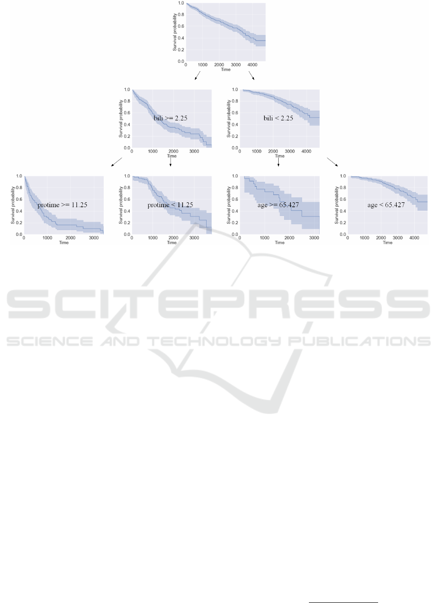
Figure 2: Example of a constructed decision tree of depth 2 with visualization of the survival function estimate at each node.

The tree is based on the following features: bili (serum bilirubin), protime (standardized blood clotting time), age.

1. A bootstrap sample of a predeﬁned size (speci-

ﬁed as a hyperparameter) is constructed, all ob-

servations have equal probability to be selected.

The part of observations out of bootstrap sample

is named as OOB.

2. Based on the approach proposed in subsection 3.2,

a decision tree is built on the boostrap sample.

3. Calculates the OOB-error of the ensemble before

and after adding the next decision tree model. The

error is calculated similarly to the RSF 2.2 model:

the prediction for observation x is the aggregation

of tree predictions for which x ∈ OOB

. The error

calculation metric is speciﬁed as a hyperparame-

ter.

4. If the added model increases the ensemble error,

the model is deleted from ensemble, and the con-

struction is terminated. Otherwise, the algorithm

returns to step 1

5. Also, the algorithm may work in a tolerance

mode: an ensemble of decision trees are sequen-

tially built for a predetermined number of models

N, OOB-error is calculated at each iteration, and

the ﬁnal number of models in the ensemble is de-

termined by the minimum error over all iterations.

The bagging model prediction is the aggregation

of model predictions in the ensemble (median, mean,

or weighted mean can be used). In particular, the

survival function is computed as an aggregation over

each time point.

To control for computational complexity, the fol-

lowing parameters are used: maximum number of

trees in the ensemble, bootstrap sample size, toler-

ance mode ﬂag, the method of aggregation of ensem-

ble model predictions, metric for calculating OOB er-

ror, parameters of singlr tree growth control.

4 EXPERIMENTS

4.1 Metrics

In this paper, we use Concordance index and In-

tegrated Brier Score metrics to evaluate the perfor-

mance of the proposed prediction models and to com-

pare them with existing ones. The Concordance Index

(Harrell Jr et al., 1996) is widely used in survival anal-

ysis. It is similar to AUC in the sense that it measures

the fraction of concordant or correctly ordered pairs

of samples among all available pairs in the dataset.

The highest value of the metric is one (if the order is

perfect), and the value of 0.5 means that the model

produces completely random predictions.

The following formula is used for calculating the

concordance index:

CI =

∑

i, j

· 1

<η

∑

i, j

Survival Analysis Algorithms based on Decision Trees with Weighted Log-rank Criteria

137

where T

is the true time of the event, and η

is the

time predicted by the model.

However, this metric is based only on the pre-

dicted time of the event, and it does not allow esti-

mating the survival function. The value of CI does not

change when the survival function is biased, although

the predicted time is highly distorted compared to the

true time.

To eliminate this problem, we use a metric called

Integrated Brier Score (Murphy, 1973), (Brier and

Allen, 1951), (Haider et al., 2020) based on the devi-

ation of the predicted survival function from the true

one (equal to 1 before the event occurs and 0 after

that). The Brier Score (BS) metric (Brier and Allen,

1951) is used for estimating the performance of the

prediction at a ﬁxed time point t and is calculated in

the following way:

BS(t) =

∑

(

(0 − S(t, x

))

if T

≤ t

(1 − S(t, x

))

if T

> t

(2)

where S(t, x

) is the prediction of the survival function

at time t for observation x

with event time T

Next, the squares of variance are averaged over

all observations at time t. The best BS value is 0,

in the case the predicted and true survival functions

coincide. However, 2 does not take into account the

censoring. In such a case, the following modiﬁcation

of the BS (Murphy, 1973),(Haider et al., 2020) can be

used:

BS(t) =

∑











(0−S(t,x

))

G(T

)

if T

≤ t, δ

= 1

(1−S(t,x

))

G(t)

if T

> t

0 if T

= t, δ

= 0

(3)

As in (2), S(t, x

) is a prediction of the survival

function at time t for observation x

with event time T

The parameter δ

in (3) is the censored ﬂag of obser-

vation x

, it is equal to 1 if the event occurred and 0 if

the event is censored. The function G(t) = P(c > t) is

the Kaplan-Meier estimation of the survival function

constructed on the censored observations (the cen-

sored ﬂag is reversed when constructing the estimate).

The squares of variance in (3) are adjusted by weight-

ing inverse probability of non-censoring:

G(T

)

if the

event occurs before t, and

G(t)

if the event occurs af-

ter t. Observations censored before t are not used in

calculation.

To aggregate the BS estimates over all time mo-

ments, the Integrated Brier Score is used:

IBS =

max

BS(t)d t

4.2 Datasets

In the experiments we use the following public medi-

cal benchmark datasets.

The Primary Biliary Cirrhosis (PBC) dataset (Ka-

plan, 1996) was collected in the time period from

1974 to 1984. The death is considered as the event.

The dataset contains 276 observations and 17 features

including cirrhosis status, treatment strategy, and clin-

ical measures. Also, 12 features such as treatment

strategies and clinical indicators may be missed, with

the maximum number of missings in the cholesterol

indicator (134 missings) and in the triglyceride indi-

cator (136 missings). At the end of the study, there

were 263 patients for whom there were no fatal out-

comes.

The German Breast Cancer Study Group (GBSG)

(Schumacher, 1994) dataset was collected in the pe-

riod from 1984 to 1989. The cancer relapse is consid-

ered as the event. The data set contains 686 observa-

tions and 8 features such as tumor characteristics and

treatment strategies. The dataset does not have miss-

ings. At the end of the study there were 387 patients

without relapse.

4.3 Experimental Setup

For honest estimating of the models performance, we

implemented hyperparameters grid search using 5-

folds cross validation (Refaeilzadeh et al., 2009). All

variable hyperparameters and their grid characteris-

tics are presented in the table 1. The best vector of

hyperparameters for the model is selected according

to the minimum value of cross-validated IBS metric.

4.4 Results

For the existing methods we used scikit-survival li-

brary (P

olsterl, 2020) implementation. For the pro-

posed methods we implemented our own code. The

results of performance estimating for all methods by

CI, IBS metrics on PBC and GBSG datasets are pre-

sented in tables 2, 3 (top 3 models by each metric are

marked in bold).

On the PBC dataset the Gradient Boosting Sur-

vival Analysis method showed the best C I, but pro-

posed in the paper Bagging Wilcoxon and Bagging

Tarone-Ware methods are next and close to the leader.

Moreover, on IBS metric proposed Bagging Peto and

Bagging Tarone-Ware methods outperformed others.

That is important, because IBS metric is more ap-

propriate for evaluating the performance of survival

analysis models since it estimates the deviation of the

predicted survival function from the true one. On

ICPRAM 2022 - 11th International Conference on Pattern Recognition Applications and Methods

138

Table 1: Hyperparameters of predictive models.

Predictive

model

Hyperparameter Values

CoxPH Sur-

vival Analy-

sis

regularization

penalty

0.1, 0.01, 0.001

ties breslow, efron

Survival Tree split strategy best, random

max depth 10 to 30 step 5

min sample leaf 1 to 20 step 1

max features sqrt, log2, None

Random Sur-

vival Forest

num estimators 10 to 100 step

max depth 10 to 30 step 5

min sample leaf 1 to 20 step 1

max features sqrt, log2, None

Gradient

Boosting SA

num estimators 10 to 100 step

max depth 10 to 30 step 5

min sample leaf 1 to 20 step 1

max features sqrt, log2, None

loss function coxph, squared,

ipcwls

learning rate 0.01 to 0.5 step

0.01

Tree max depth 10 to 30 step 5

min sample leaf 1 to 20 step 1

signiﬁcance

threshold

0.01, 0.05, 0.1,

0.15

Bagging bootstrap sample

size

0.3 to 0.9 step

0.1

num estimators 10 to 50 step 5

max depth 10 to 30 step 5

min sample leaf 1 to 20 step 1

Table 2: PBC dataset results.

Predictive model CI IBS

Survival Tree 0.61325 0.25292

Gradient Boosting Sur-

vival Analysis

0.65536 0.23480

CoxPH Survival Analy-

sis

0.63965 0.23050

Random Survival Forest 0.65060 0.20516

Tree tarone-ware 0.64744 0.26982

Tree wilcoxon 0.64443 0.25092

Tree logrank 0.63582 0.23240

Tree peto 0.64001 0.21770

Bagging wilcoxon 0.65284 0.21341

Bagging logrank 0.63783 0.20829

Bagging peto 0.64988 0.20258

Bagging tarone-ware 0.65118 0.20104

the GBSG dataset all proposed Bagging methods out-

performed their existing competitors by both CI, IBS

metrics.

Table 3: GBSG dataset results.

Predictive model CI IBS

Survival Tree 0.58500 0.19119

Gradient Boosting Sur-

vival Analysis

0.60818 0.17768

Random Survival Forest 0.61795 0.17352

CoxPH Survival Analy-

sis

0.61281 0.17324

Tree logrank 0.58162 0.19082

Tree peto 0.59781 0.18582

Tree wilcoxon 0.59192 0.18510

Tree tarone-ware 0.60029 0.18489

Bagging logrank 0.61861 0.17262

Bagging wilcoxon 0.62707 0.17157

Bagging tarone-ware 0.62276 0.17112

Bagging peto 0.62252 0.17079

Also, it is important to note that in many cases the

proposed single-model decision trees with weighted

long-rank criteria outperform their single-model com-

petitors such as Survival tree and Cox PH regularized

regression.

Consequently, the best prediction models for both

datasets are based on bagging ensembles of decision

trees with weighted log-rank split criteria.

5 CONCLUSIONS

In this paper, we have proposed a method for build-

ing nonlinear survival models based on the recursive

partitioning with weighted log-rank test as a split cri-

terion. This approach allows avoid some disadvan-

tages of the existing state-of-the-art methods in sur-

vival analysis and build survival models that do not

exploit such assumptions as proportionality of haz-

ards over time and linear dependence between the log

of hazard and combination of covariates. Besides, the

proposed method effectively works with missing val-

ues, can pay greater attention to the events with ear-

lier occurrence time. Using Bonferroni adjustment for

weighted log-rank in splitting procedure allows more

correct comparisons among candidate features with

different power. We have also experimentally shown

on medical becnchmark datasets that the bagging en-

sembles of the proposed models outperform the ex-

isting models and their ensembles in terms of the

Concordance index and Integrated Brier Score met-

rics. In further research, we plan to study the behav-

ior of boosting ensembles of the proposed models, to

develop efﬁcient algorithms for time-efﬁcient ﬁnding

the optimal split with weighted log-rank criteria for

high-power categorical features and on large dataset,

Survival Analysis Algorithms based on Decision Trees with Weighted Log-rank Criteria

139

as well as to investigate the performance of the pro-

posed methods on other benchmark datasets, includ-

ing cases from other application areas.

REFERENCES

Aster, R. C., Borchers, B., and Thurber, C. H. (2018). Pa-

rameter estimation and inverse problems. Elsevier.

Benjamini, Y. and Hochberg, Y. (1995). Controlling the

false discovery rate: a practical and powerful ap-

proach to multiple testing. Journal of the Royal statis-

tical society: series B (Methodological), 57(1):289–

300.

Breslow, N. (1970). A generalized kruskal-wallis test for

comparing k samples subject to unequal patterns of

censorship. Biometrika, 57(3):579–594.

Brier, G. W. and Allen, R. A. (1951). Veriﬁcation of weather

forecasts. In Compendium of meteorology, pages 841–

848. Springer.

Buyske, S., Fagerstrom, R., and Ying, Z. (2000). A class

of weighted log-rank tests for survival data when the

event is rare. Journal of the American Statistical As-

sociation, 95(449):249–258.

Ciampi, A., Thiffault, J., Nakache, J.-P., and Asselain, B.

(1986). Stratiﬁcation by stepwise regression, corre-

spondence analysis and recursive partition: a compar-

ison of three methods of analysis for survival data with

covariates. Computational statistics & data analysis,

4(3):185–204.

Cox, D. R. (1972). Regression models and life-tables. Jour-

nal of the Royal Statistical Society: Series B (Method-

ological), 34(2):187–202.

Friedman, J. H. (2001). Greedy function approximation: a

gradient boosting machine. Annals of statistics, pages

1189–1232.

Haider, H., Hoehn, B., Davis, S., and Greiner, R. (2020). Ef-

fective ways to build and evaluate individual survival

distributions. J. Mach. Learn. Res., 21:85–1.

Harrell Jr, F. E., Lee, K. L., and Mark, D. B. (1996).

Multivariable prognostic models: issues in develop-

ing models, evaluating assumptions and adequacy, and

measuring and reducing errors. Statistics in medicine,

15(4):361–387.

Hothorn, T., B

uhlmann, P., Dudoit, S., Molinaro, A., and

Van Der Laan, M. J. (2006). Survival ensembles. Bio-

statistics, 7(3):355–373.

Ishwaran, H., Kogalur, U. B., Blackstone, E. H., and Lauer,

M. S. (2008). Random survival forests. The annals of

applied statistics, 2(3):841–860.

Kaplan, E. L. and Meier, P. (1958). Nonparametric esti-

mation from incomplete observations. Journal of the

American statistical association, 53(282):457–481.

Kaplan, M. M. (1996). Primary biliary cirrhosis. New Eng-

land Journal of Medicine, 335(21):1570–1580.

Klein, J. P. and Moeschberger, M. L. (1997). Statistics

for biology and health. Stat. Biol. Health, New York,

27238.

LeBlanc, M. and Crowley, J. (1993). Survival trees by good-

ness of split. Journal of the American Statistical As-

sociation, 88(422):457–467.

Lee, S.-H. (2021). Weighted log-rank statistics for acceler-

ated failure time model. Stats, 4(2):348–358.

Lin, D. (2007). On the breslow estimator. Lifetime data

analysis, 13(4):471–480.

Morgan, J. N. and Sonquist, J. A. (1963). Problems in the

analysis of survey data, and a proposal. Journal of the

American statistical association, 58(302):415–434.

Murphy, A. H. (1973). A new vector partition of the proba-

bility score. Journal of Applied Meteorology and Cli-

matology, 12(4):595–600.

Nelson, W. (1972). Theory and applications of hazard

plotting for censored failure data. Technometrics,

14(4):945–966.

Peto, R. and Peto, J. (1972). Asymptotically efﬁcient rank

invariant test procedures. Journal of the Royal Statis-

tical Society: Series A (General), 135(2):185–198.

olsterl, S. (2020). scikit-survival: A library for time-to-

event analysis built on top of scikit-learn. J. Mach.

Learn. Res., 21(212):1–6.

Refaeilzadeh, P., Tang, L., and Liu, H. (2009). Cross-

validation. Encyclopedia of database systems, 5:532–

538.

Schumacher, M. (1994). Rauschecker for the german breast

cancer study group, randomized 2× 2 trial evaluating

hormonal treatment and the duration of chemotherapy

in node-positive lbreast cancer patients. Journal of

Clinical Oncology, 12:2086–2093.

Tarone, R. E. and Ware, J. (1977). On distribution-free

tests for equality of survival distributions. Biometrika,

64(1):156–160.

ICPRAM 2022 - 11th International Conference on Pattern Recognition Applications and Methods

140