Multi-periodic Joint Replenishment Planning Method for Various

All-unit Discounts

Agathe Métaireau

1,2

, Rabin Sahu

, Simon Delecourt

, Alexandre Gerussi

and Manuel Davy

Vekia, 143 rue d’Athènes, Lille, France

Univ. Lille, CNRS, Centrale Lille, UMR 9189 - CRIStAL, France

Keywords:

Joint Replenishment, Multi-period Planning, Inventory Control, Integer Linear Programming.

Abstract:

This paper aims at developing a multiperiodic joint replenishment optimization method to tackle all-unit dis-

counts. In many industrial contexts, there exist multi-item constraints that can’t be treated by single-item

optimization. For example, suppliers can charge a ﬁxed ordering cost or offer a discount above a given or-

dered quantity. To tackle such constraints, we set in place a model based on ordering blocks. This modeling

enables to reduce the search-space by predetermining a given set of possible order quantities. The model is

then solved using an Integer Linear Program that outputs the ordering plan for a given time horizon. This Inte-

ger Linear Program searches for the ordering block combination that gives the minimal cost. The cost function

includes single-item costs like purchase or inventory costs as well as multi-item costs. The methodology was

tested on twenty generated instances and compared with a single-period single-item replenishment engine. We

show that our multiperiodic joint replenishment approach allows a reduction of the costs and an increase in

the service level.

1 INTRODUCTION

A large part of the research conducted on inventory

replenishment planning focuses on single-item con-

trol. In many references, the target is to ﬁnd the best

policy and its parameters. The ﬁnal goal is to reach

optimal or near-optimal inventory control for given

situations and different objectives. There are however

several industrial contexts where treating items sepa-

rately is not the best strategy. In these contexts, there

exist interactions between items. Fixed ordering cost

or all-unit and incremental discounts are examples of

this aspect. In such contexts, the problem cannot be

reduced to several single-item sub-problems, because

the constraints apply to the whole order. In this paper,

we will only consider ﬁrst-order interactions between

the items, which can happen in various situations, in

addition to the ones we mentioned above.

As this type of problem cannot be decomposed,

there is a need to develop strategies to jointly replen-

ish the items under control. Moreover, reaching all-

unit or incremental discounts sometimes requires or-

dering more than the optimal quantity we compute for

one coverage period, and considering several periods

is a way to reach the discounts with relevant order-

ing quantities, which is an incentive to consider multi-

periodic replenishment planning.

As a result, we will consider in this article a

multi-item multi-period replenishment problem, with

a ﬁxed cost constraint and for various types of all-

unit discounts. The multi-periodic joint replenish-

ment problem has already been addressed in the lit-

erature for different contexts. Some authors calcu-

late the Economic Order Quantity for this context,

like (Das et al., 2000), who use geometric program-

ming and gradient-based non-linear programming on

capacitated systems and (Mousavi et al., 2013), who

show the performance of a genetic algorithm with

a mix of incremental and all-unit discount. (Man-

dal et al., 2011) use fuzzy techniques and genetic al-

gorithms to address the optimal production control

problem with the demand rate being stock-dependent.

(Rezaei and Davoodi, 2008) use genetic algorithms

in the context of defective items with supplier selec-

tion. (Gao et al., 2020) use dynamic programming

to ﬁnd a multi-raw material control policy under car-

bon emission constraints. (Mirzapour Al-e-Hashem

and Rekik, 2014) developed a Mixed-Integer Linear

Program (MILP) to solve an inventory routing prob-

lem with deterministic demand and transshipment al-

lowed.

The multi-period joint replenishment problem is

NP-Hard ((Sahu, 2020)). Therefore, it is impossible

Métaireau, A., Sahu, R., Delecourt, S., Gerussi, A. and Davy, M.

Multi-periodic Joint Replenishment Planning Method for Various All-unit Discounts.

DOI: 10.5220/0010986800003117

In Proceedings of the 11th International Conference on Operations Research and Enterprise Systems (ICORES 2022), pages 86-93

ISBN: 978-989-758-548-7; ISSN: 2184-4372

to solve it exactly in a reasonable time, and it is nec-

essary to solve it approximately. In this article, we

tried to reduce the solution space of the problem we

address by modeling. In this model, the orders we

can place are represented by objects we call "order-

ing blocks", as deﬁned in (Sahu, 2020). The opti-

mization aims to ﬁnd the best combination of blocks

for the considered horizon. It enabled us to formu-

late the problem we want to solve as an Integer Linear

Program (ILP) and to solve it using a classic branch-

and-bound solver. As there are multiple cases of all-

unit discounts in industrial replenishment contexts,

the ILP has been written to be generic and applica-

ble to a large set of discount types.

The ILP allows an easy formulation of the prob-

lem. As free and commercial solvers already exist,

there is no need to develop more complicated heuris-

tics to solve ILPs. As a result, the method we offer

is easily implementable in real multiperiodic joint-

replenishment contexts. Moreover, the optimization

tool we develop is intended to be a module assisting a

single-item single-period replenishment optimization

engine. Therefore, it is suitable to be integrated with

already existing optimization tools.

The remainder of the paper is organized as fol-

lows. We will ﬁrst describe the approach we devel-

oped and the notations we use in section 2. Then, we

will present the ILP in section 3. We will next de-

scribe the experimental protocol we put in place to

validate the model and present the numerical results

in section 4. Finally, we will provide a conclusion in

section 5.

2 DEVELOPED APPROACH AND

NOTATIONS

In this section, we will ﬁrst detail the problem we ad-

dress and give some examples of application in indus-

trial replenishment contexts. Then, we will explain

the approach we put in place to model and solve it.

2.1 Details of the Problem and Use

Cases

As we stated before, we focus on constraints concern-

ing several items at the same time. It implies a need to

design an optimization method that takes into account

all the items simultaneously. We search to plan the re-

plenishment for groups of items jointly, on several pe-

riods for a ﬁnite horizon, considering joint costs and

discounts. In this paper, we consider only all-unit dis-

counts. This means the discount is applied on all the

items ordered once the breakdown is reached. We ap-

ply a direct grouping strategy, as deﬁned in (Bastos

et al., 2017), and consider only groups of items that

have the same cycle time.

There are two major categories of multi-item con-

straints we consider: ﬁxed ordering cost and all-unit

discount. They are deﬁned as follows.

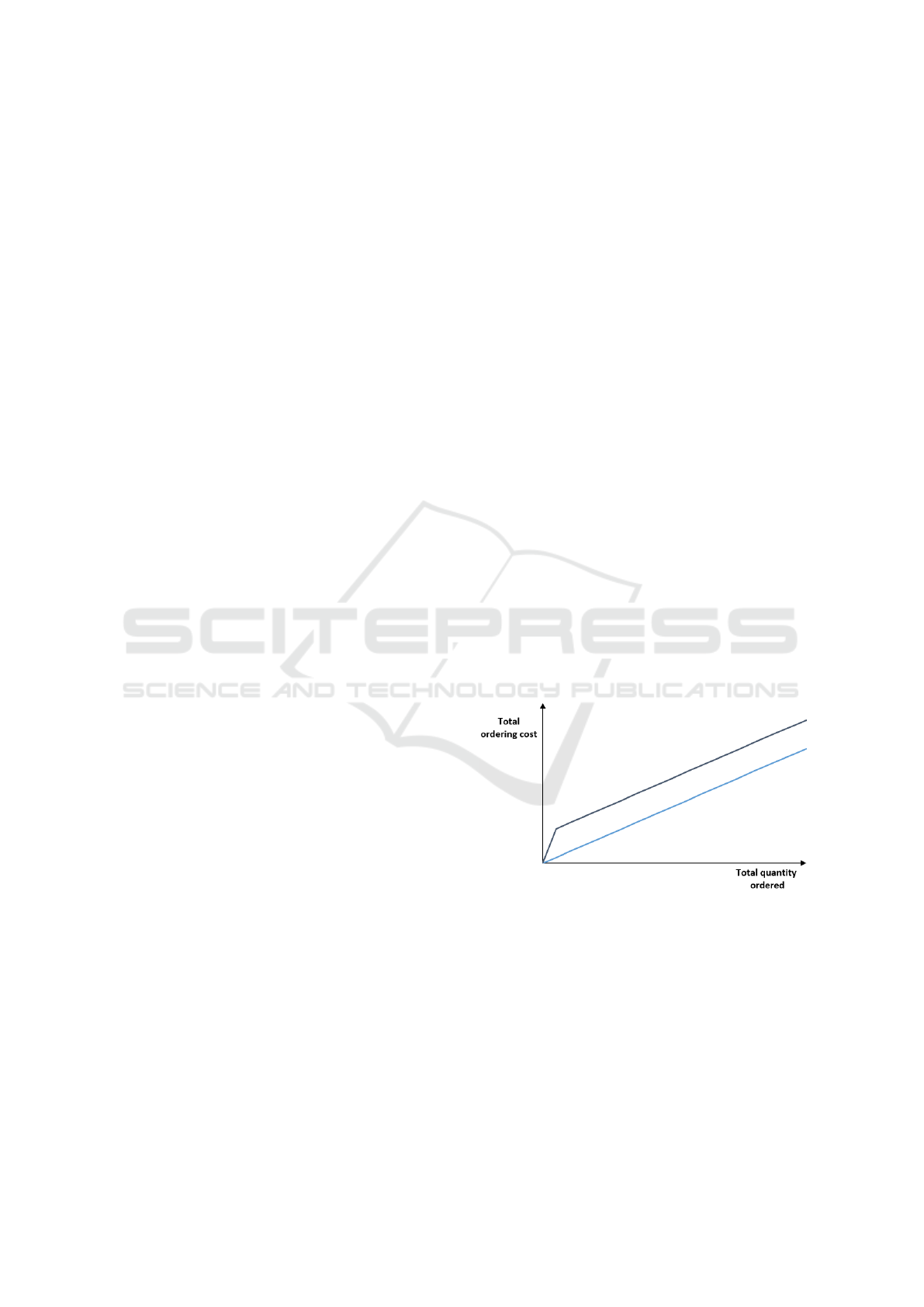
Fixed Ordering Cost: It is a cost applied to the

whole order once we order something (i.e. when

the total quantity ordered is strictly superior to 0).

For example, a supplier can add a transport cost

to the ordering cost, and this cost is only applied

if something is ordered. This cost is also called in

the literature "Major Ordering Cost".

All-unit Discount: It is a discount applied on all the

items ordered (i.e. on the total ordering cost)

once a given breakdown is reached. There can

be one or several breakdowns with corresponding

discounts. The breakdowns can also concern dif-

ferent values, such as the total ordering cost or the

total quantity ordered, but also the total weight or

volume of the order for example. A practical ex-

ample of the all-unit discount is the Franco, where

the supplier charges a constant penalty cost if the

total ordering cost is lower than a given break-

down.

Figures 1 and 2 are graphical examples of the two

notions explained above.

Figure 1: Representation of the cost function in case of a

ﬁxed ordering cost. The dark blue curve is the case without

ﬁxed ordering cost.

2.2 Modeling Approach and Deﬁnitions

As the problem is NP-Hard, we can’t expect to ﬁnd

the optimal solution to large-scale instances in a rea-

sonable time. Therefore, we have to deﬁne a pro-

cess to ﬁnd good-quality solutions in a suitable de-

lay. In this article, we choose to reduce the search

space by modeling. First, we constrain the time steps

Multi-periodic Joint Replenishment Planning Method for Various All-unit Discounts

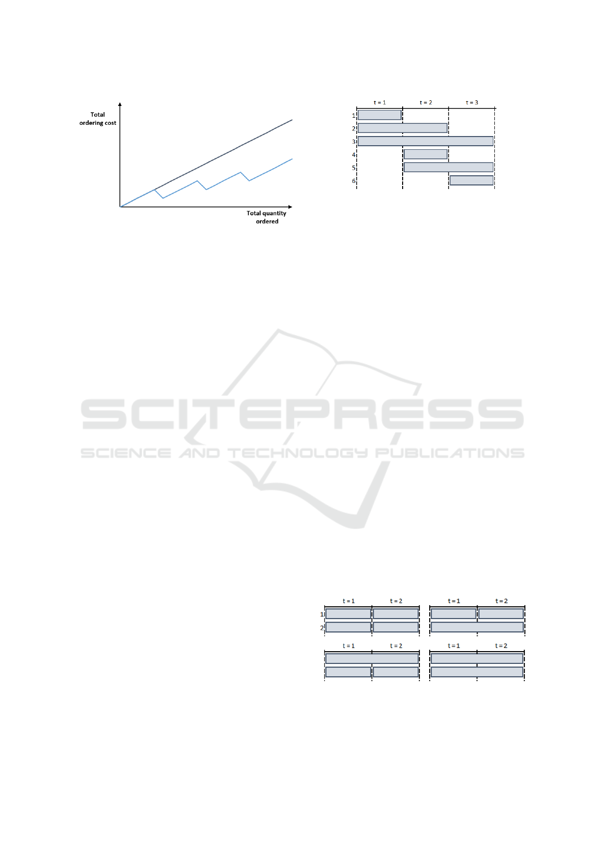
Figure 2: Representation of the cost function for an all-unit

discount with three breakdowns and three corresponding

ﬁxed discounts. The dark blue curve is the case without

any discount.

at which an order can be placed. It seems to be a rea-

sonable choice, as the ordering dates are frequently

constrained in real-life replenishment contexts.

We deﬁne the notion of coverage period as a time

interval [t

, t

] for which an order can be placed at t

and no order can be placed until t

. In other words,

this is the smallest possible interval between two or-

ders.

We also choose to constrain the quantities that can

be ordered. At the beginning of every coverage pe-

riod, the decision-maker can only choose among a set

of possible ordering quantities. These quantities are

the optimal ordering quantities for t coverage periods,

with t going from 1 to the end of the planning horizon.

They are calculated before the multi-periodic joint re-

plenishment optimization.

As a result, we represent the possible orders as an

object called "block". Every block contains several

attributes. First, it has a length, which is the num-

ber of coverage periods it encompasses. It has then a

quantity to order, which is the precomputed optimal

quantity for the block’s length, and a cost, which is

the total cost incurred for ordering the optimal quan-

tity. The block’s cost involves the purchase cost, the

holding cost, the lost-sale or backorder cost, and any

relevant cost for the problem under study. A block

can also contain another attribute named value, which

represents the value compared to the discount break-

down. This value can be the purchase cost, the vol-

ume, the weight, etc. Figure 3 represents all the pos-

sible blocks for one item and a time horizon of three

coverage periods.

2.3 Notations

In this section, we describe the notations we use in

the remainder of the article. All the notations we will

use are listed below. The subscripts t refer to the time

Figure 3: Possible blocks for one item and a time horizon

of three coverage periods.

steps, n to the items, and i to the cost breakdowns.

T - Time horizon

N - Size of the item set

I - Number of cost breakdowns

K - Fixed ordering cost

- Block corresponding to the order of item n

from coverage period starting at t

and ending at t

- Quantity to order for the block B

- Cost incurred by the block B

- Value of the block B

to be compared to

the breakdowns

- Breakdown i

- Fixed cost or discount for a total order value

under the breakdown i

- Cost or discount per unit for a total order value

under the breakdown i

2.4 Solution Approach

The goal of the multi-periodic joint replenishment op-

timization method we develop in this article is to ﬁnd

what quantity of each item to order at every time step

of the planning horizon while minimizing the total

cost. This total cost, which we call TC in this section,

includes the block’s cost and the costs and discounts

incurred by the multi-item constraints.

Let P

be the set of possible block combinations

for an item set of size N and a planning horizon T . As

an example, a representation of the set P

is provided

in Figure 4.

Figure 4: Representation of the set of possible block combi-

nation for two items and a planning horizon of two periods.

Given N and T , each possible block combination

p in P

has a total cost TC(p), which is the sum of

ICORES 2022 - 11th International Conference on Operations Research and Enterprise Systems

the costs of the blocks selected in p and the corre-

sponding multi-item costs and discount. To ﬁnd the

best replenishment planning in this context, we are

looking for the block combination p

∗

with the mini-

mum cost, as described in the equation 1.

∗

= arg min

p∈P

TC(p) (1)

In the next section, we will describe the method-

ology we use to ﬁnd p

∗

3 OPTIMIZATION

METHODOLOGY

An intuitive solution to solve the problem we de-

scribed above would be to generate every possible

block combination, compute their respective total

cost, and choose the one with the lowest total cost.

However, the number of possible block combinations

for a time horizon T and an item set of size N is

N×T −1

. It means the number of possible block com-

binations quickly increases with the growth of both T

and N. For example, if T = 5 and N = 5, there are 1

048 576 possibilities, which illustrates how the brute

force approach rapidly becomes intractable.

To tackle this, we chose to solve the problem by

using an Integer Linear Program (ILP). This optimiza-

tion method has the advantage of being easy to formu-

late, implement, and solve using commercial or free

solvers.

We will present the formulation of the ILP in the

next sections. Section 3.1 lists the data used in the

ILP, Section 3.2 details its variables. Section 3.3 is

dedicated to the objective. Section 3.4 lists all the

constraints and provide some explanation of them.

Section 3.5 details the domains of the variables.

3.1 Data

T - Time horizon

N - Set of items

I - Number of breakdowns

K - Fixed ordering cost

M - Suitably large number

∀n ∈ N, ∀t

∈ J1, T K, ∀t

∈ J1, T K, C

- Cost of the

block B

∀n ∈ N, ∀t

∈ J1, T K, ∀t

∈ J1, T K, V

- Value of

the block B

∀i ∈ J1, IK, l

- i-th breakdown

∀i ∈ J1, I +1K, f

- Fixed cost or discount correspond-

ing to a value ordered over l

i−1

and under l

∀i ∈ J1, I + 1K, u

- Cost or discount per unit corre-

sponding to a value ordered over l

i−1

and under l

3.2 Variables

∀n ∈ N, ∀t

∈ J1, T K, ∀t

∈ J1, T K,

1 i f the block B

is selected

0 otherwise

∀t ∈ J1, T K,

1 i f the value ordered is 0

0 otherwise

∀t ∈ J1, T K,



1 i f the value ordered is

strictly between 0 and l

0 otherwise

∀t ∈ J1, T K, ∀i ∈ J3, IK



1 i f the value ordered is between

i−1

and l

excluded

0 otherwise

∀t ∈ J1, T K,

tI+1



1 i f the value ordered is greater

than l

0 otherwise

∀t ∈ J1, T K, ∀i ∈ J1, I + 1K

Value ordered at t i f η

= 1

0 otherwise

3.3 Objective

min

∑

n∈N

∑

t=1

K(1 − η

)

∑

i=1

+ f

)

3.4 Constraints

∀n ∈ N, ∀t

∈ J1, T K, ∀t

∈ J1, T K,

6 t

(2)

∀n ∈ N,

∑

−t

+ 1)x

= T (3)

∀n ∈ N,

∑

t=1

ntT

= 1 (4)

Multi-periodic Joint Replenishment Planning Method for Various All-unit Discounts

∀n ∈ N, ∀t ∈ J1, T − 1K,

∑

nt+1t

(5)

∀t ∈ J1, T K, M (1 − η

) >

∑

n∈N

∑

ntt

(6)

∀t ∈ J1, T K, (1 − η

) 6

∑

n∈N

∑

ntt

(7)

∀t ∈ J1, T K, ∀i ∈ J2, I + 1K,

i−1

∑

n∈N

∑

ntt

(8)

∀t ∈ J1, T K, ∀i ∈ J2, IK,

M(1 − η

) >

∑

n∈N

∑

ntt

+ ε (9)

∀t ∈ J1, T K,

I+1

∑

i=1

= 1 (10)

∀t ∈ J1, T K, ∀i ∈ J1, I + 1K,

∑

n∈N

∑

ntt

) − M(1 − η

) (11)

∀t ∈ J1, T K, ∀i ∈ J1, I + 1K,

∑

n∈N

∑

ntt

(12)

∀t ∈ J1, T K, ∀i ∈ J1, I + 1K, y

6 Mη

(13)

Constraint 2 ensures that we select only blocks

for which the starting coverage period is lower than

or equal to the ending coverage period. Constraint 3

ensures the entire planning horizon is covered. Con-

straints 4 and 5 ensure that the blocks we select do not

overlap. Constraints 6, 7, 8, and 9 rule the value of η

according to its deﬁnition. If the total value ordered

can be lower than 1, it is necessary to add a "+ε" at

the end of the right part of constraint 7 to ensure its

good functioning. The "+ε" at the end of the left part

of constraint 9 allows having the behavior of a strict

inequality. Constraint 10 ensures only one η

is se-

lected each period. Constraints 11, 12, and 13 rule

the value of y

according to its deﬁnition.

3.5 Domains

∀n ∈ N, ∀t

∈ J1, T K, ∀t

∈ J1, T K, x

∈ {0, 1}

∀t ∈ J1, T K, ∀i ∈ J1, IK, η

∈ {0, 1}

∀t ∈ J1, T K, ∀i ∈ J1, IK, y

∈ N

The domain of y

is consistent with the unit of

V . We consider the case where V only takes integer

values, but if V takes continuous values, the Integer

Linear Program becomes a Mixed Integer Linear Pro-

gram (MILP).

4 EXPERIMENTATIONS AND

COMPUTATIONAL RESULTS

To evaluate the interests of multiperiodic joint replen-

ishment planning and the performance of the method

we developed, we chose to compare it with a single-

period single-item optimization method. We used a

single-period single-item ordering engine as a base-

line for our experimentations. This engine uses a

sample-based optimization approach for stochastic re-

plenishment planning. Given a set ov demand sam-

ples, this engine aims to ﬁnd the optimal quantity

to order on a ﬁxed coverage period. It will mini-

mize the so-called "coverage period cost", which is

the expected cost on the whole period, and includes

the holding cost, the lost-sale cost, and an potential

single-item ﬁxed cost. The optimal quantity is found

by using an enumerativesearch heuristic, described in

(Sahu, 2020).

Both order engines are compared on the total cost

performance criterion, which includes the purchase

cost, the inventory cost, the shortage cost, and the

multi-item cost. In the experiments, the multi-item

constraint is a Franco penalty, as described in the sec-

tion 2.1, so the multi-item cost includes only eventual

Franco penalties.

To conduct experiments, we generated twenty dif-

ferent instances, each containing ten items. We as-

sume perfect forecast, i.e. we assume that we per-

fectly know the demand distribution of the items. In

every instance, all the demand distributions of the

items are stationary Poisson distribution, and we as-

sume all the unmet demand is lost. The parameters of

the instances we used are detailed in the tables 1 and

2. The Integer Linear Program has been implemented

using the PuLP library in Python, and solved using

the COIN-OR Branch and Cut (CBC) solver.

ICORES 2022 - 11th International Conference on Operations Research and Enterprise Systems

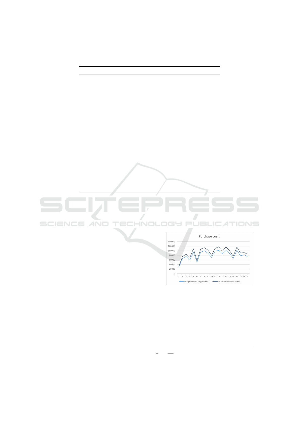
Table 1: Details of the instances used for the experiments. λ

represents the mean of the Poisson distribution for the demand

of the i-th item of the instance. The global parameters are the purchase cost p = 5, storage cost h = 0.1 and lost sale cost

w = 10.

Instance n

◦

1 10 10 10 10 10 10 10 10 10 10

2 13 25 14 15 41 12 20 34 19 34

3 39 44 13 21 15 47 31 14 29 8

4 45 39 20 11 11 9 9 10 42 10

5 24 30 14 34 42 35 24 35 40 46

6 18 17 14 32 22 23 7 11 11 19

7 47 33 50 25 48 38 16 11 18 33

8 39 47 41 26 31 28 13 32 47 36

9 30 6 17 18 34 50 46 48 50 10

10 36 26 14 18 48 11 44 21 15 16

11 24 41 42 37 22 26 45 7 42 49

12 50 46 48 43 16 13 46 6 38 42

13 20 48 13 20 41 48 15 36 6 48

14 21 34 18 47 29 31 44 44 34 44

15 38 44 22 25 38 42 9 49 5 30

16 22 11 13 36 15 20 35 43 31 7

17 37 38 12 18 45 49 47 30 46 31

18 44 15 18 8 45 30 10 21 36 41

19 19 31 42 40 37 50 5 16 23 22

20 11 43 43 19 19 46 25 7 7 31

To compare both replenishment processes, we

used the following experimental protocol.

1. Generate demand samples for every item of the

instance and every period of the planning horizon.

2. Given initial inventory levels, launch the single-

item single-period order engine. Simulate the or-

der and demand process and update the inventory

levels.

3. Record the costs associated with the simulated pe-

riod.

4. Repeat steps 1. and 2. on the whole planning hori-

zon.

5. Compute the total cost for the single-item single-

period ordering simulation.

6. Given the same initial inventory levels, launch the

multi-period multi-item order engine. Record the

replenishment planning.

7. Simulate the order and demand process using the

same demand samples on the entire planning hori-

zon and record the costs associated with every

simulated period.

8. Compute the total cost for the multi-period multi-

item ordering simulation.

This protocol was used on the twenty instances

described above. It allowed us to compare the differ-

ent costs incurred by both optimization methods, and

conclude on the relevancy of the multiperiodic joint

replenishment planning. The comparison of the dif-

ferent costs (purchase cost, inventory cost, shortage

cost, and multi-item cost) is shown on the ﬁgures 5 to

8. The averaged savings are displayed in the table 3.

Figure 5: Comparison of the purchase costs given by the

single-period single-item and multi-period multi-item ap-

proaches on all the instances.

The values displayed in table 3 are deﬁned as fol-

lows. For a given cost type, let C

SPSI

and C

MPMI

be re-

spectively the total cost incurred by the single-period

single-item approach for the instance j and the total

cost incurred by the multi-period multi-item approach

on the same instance. Then, let S

= TC

SPSI

−C

MPMI

be the total savings for instance j and S

T S

SPSI

. Let

S and S

be their respective averaged values on all the

instances.

Multi-periodic Joint Replenishment Planning Method for Various All-unit Discounts

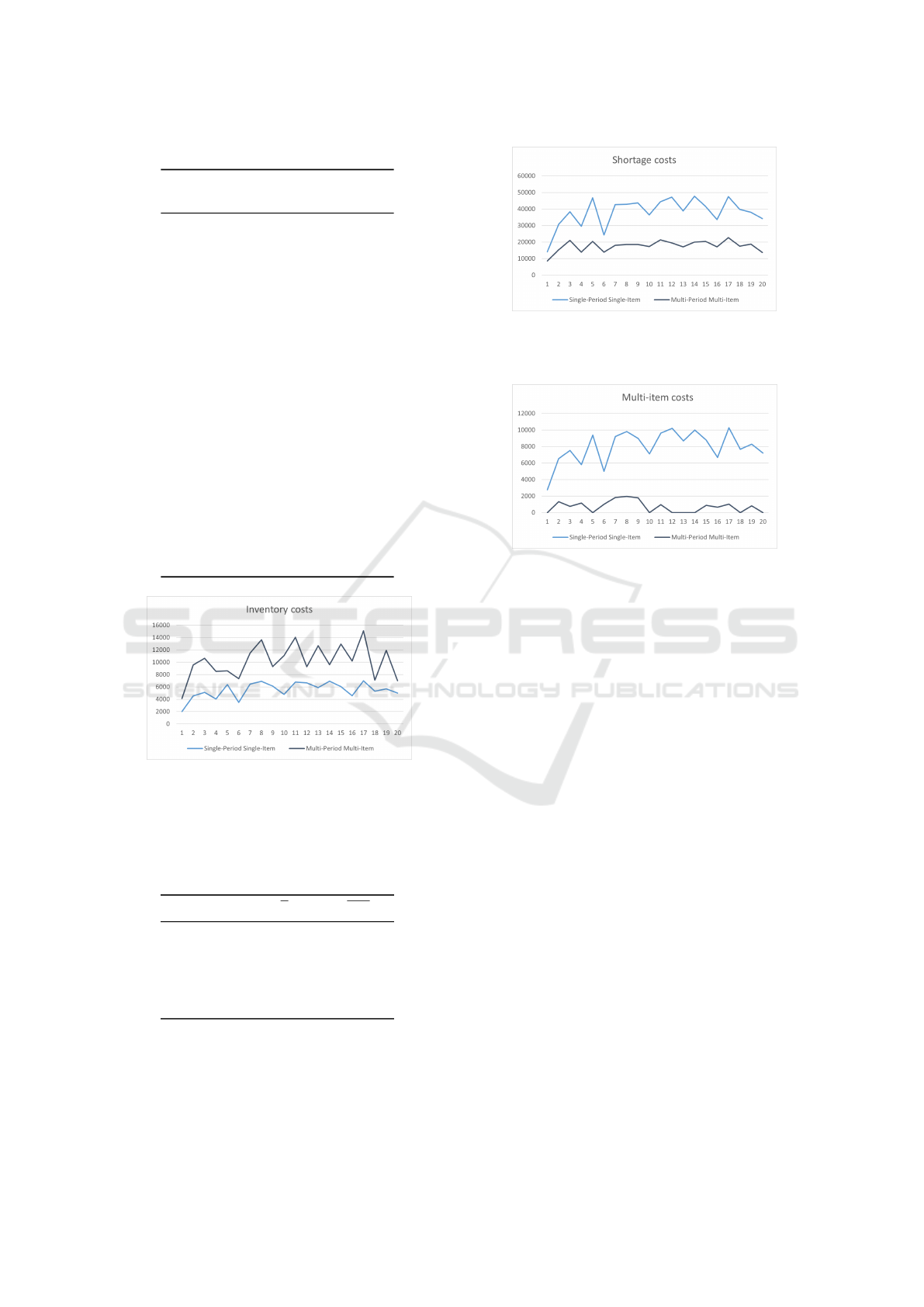
Table 2: Franco parameters of the instances.

Instance n

◦

Franco

threshold

Franco

penalty

1 800 276.35

2 2838 654

3 2250 753

4 2250 581.25

5 2150 939

6 1700 500

7 2400 920.5

8 2943 943

9 2150 899.5

10 2250 711

11 2889 963

12 2150 1019.95

13 2350 867

14 2050 999

15 2650 878.7

16 2250 668

17 3078 1025.95

18 1800 766

19 2484 828

20 1550 722.45

Figure 6: Comparison of the inventory costs given by the

single-period single-item and multi-period multi-item ap-

proaches on all the instances.

Table 3: Averaged savings obtained with the multi-period

multi-item approach compared to the single-period single-

item approach.

Cost type S S

Purchase -11255.5 -13.76%

Inventory -4725.38 -88.83%

Shortage 20427 52.72%

Multi-item 7267.32 91

Total 11714.44 8.70

Regarding the cost comparison, we obtained an

overall cost reduction of 8.70% by using the multi-

period multi-item approach. We also observe higher

purchase and inventory costs, which can be explained

by the fact that this order engine tends to order more

Figure 7: Comparison of the lost sale costs given by the

single-period single-item and multi-period multi-item ap-

proaches on all the instances.

Figure 8: Comparison of the Franco costs given by the

single-period single-item and multi-period multi-item ap-

proaches on all the instances.

than the single-period single-item one. The cost re-

duction comes from the lost sale cost and the multi-

item cost. As a result, the proposed multi-period

multi-item order engine allows to optimize the total

cost regarding the multi-item constraints, as it was de-

signed for, but it also allows to reduce lost sales, and

therefore to increase the service level.

5 CONCLUSION AND FUTURE

RESEARCH

In this paper, we present a method to optimize inven-

tory replenishment by taking into account multi-item

constraints. We develop a multi-period multi-item op-

timization tool to answer this problem. As the multi-

periodic joint replenishment planning is an NP-Hard

problem, we approximate the problem by modeling,

to obtain good solutions in a reasonable time. To re-

duce the search-space, we introduced the concept of

ordering blocks. This approximation seems to be rele-

vant because it is in line with industrial ordering pro-

cesses, and still adaptable to various situations. We

wrote an Integer Linear Program to ﬁnd the optimal

combination of blocks by minimizing the sum of the

single-item costs (purchase, inventory, and shortage

costs) and the multi-item costs (ﬁxed ordering cost,

ICORES 2022 - 11th International Conference on Operations Research and Enterprise Systems

Franco costs, discounts). This Integer Linear Program

has been developed in the purpose to be adaptable to

various all-unit discounts.

This multi-period multi-item approach was com-

pared with a single-period single-item order engine.

Using twenty generated instances, the performance of

both methods was evaluated based on the costs ob-

tained by simulation using a sample of the demand.

We chose to restrict our study to stationary Poisson

demand and to a single Franco constraint, but the

model allows to treat various demand types and multi-

item constraints. We showed that the multi-period

multi-item order engine we developed incurred a re-

duction of the total cost on all the instances, espe-

cially on the multi-item costs and on the shortage cost.

Therefore, this method allows better management of

multi-item constraints and discounts and an increase

in the service level.

For further research, the model can be tested with

different discount types, like a ﬁxed ordering cost or a

ﬁxed discount, as we only tested with a Franco here. It

would also be interesting to evaluate the performances

of the method in case of the imperfect forecast, to see

how the demand uncertainty impacts the relevancy of

this approach. The model can also be extended or

adapted to tackle incremental discounts, which were

excluded in this research.

REFERENCES

Bastos, L. d. S. L., Mendes, M. L., Nunes, D. R. d. L., Melo,

A. C. S., and Carneiro, M. P. (2017). A systematic

literature review on the joint replenishment problem

solutions: 2006-2015. Production, 27(2008):2006–

2015.

Das, K., Roy, T. K., and Maiti, M. (2000). Multi-item inven-

tory model with quantity-dependent inventory costs

and demand-dependent unit cost under imprecise ob-

jective and restrictions: A geometric programming ap-

proach. Production Planning and Control, 11(8):781–

788.

Gao, X., Chen, S., Tang, H., and Zhang, H. (2020). Study

of optimal order policy for a multi-period multi-raw

material inventory management problem under carbon

emission constraint. Computers and Industrial Engi-

neering, 148(51705384):106693.

Mandal, S., Maity, A. K., Maity, K., Mondal, S., and Maiti,

M. (2011). Multi-item multi-period optimal produc-

tion problem with variable preparation time in fuzzy

stochastic environment. Applied Mathematical Mod-

elling, 35(9):4341–4353.

Mirzapour Al-e-Hashem, S. M. and Rekik, Y. (2014).

Multi-product multi-period Inventory Routing Prob-

lem with a transshipment option: A green ap-

proach. International Journal of Production Eco-

nomics, 157(1):80–88.

Mousavi, S. M., Hajipour, V., Niaki, S. T. A., and Alikar, N.

(2013). Optimizing multi-item multi-period inventory

control system with discounted cash ﬂow and inﬂa-

tion: Two calibrated meta-heuristic algorithms. Ap-

plied Mathematical Modelling, 37(4):2241–2256.

Rezaei, J. and Davoodi, M. (2008). A deterministic, multi-

item inventory model with supplier selection and im-

perfect quality. Applied Mathematical Modelling,

32(10):2106–2116.

Sahu, R. K. (2020). General framework and optimization

methods for stochastic replenishment planning in in-

dustrial contexts. Theses, Université de Lille.

Multi-periodic Joint Replenishment Planning Method for Various All-unit Discounts