SP4LC: A Method for Recognizing Power Consumers in a Smart Plug

aniel Istv

an N

emeth

and K

alm

an Tornai

azm

any P

eter Catholic University, F. of Information Technology and Bionics, 50/a Pr

ater str, 1083 Budapest, Hungary

Keywords:

Smart Homes, Consumer Recognition, Load Classiﬁcation, Smart Plugs, Smart Grid, Edge Computing,

Machine Learning.

Abstract:

Electrical load classiﬁcation is a crucial task related to balance management in smart electrical grids. The

classiﬁcation algorithms and methods enable the smart system to schedule and adjust the grid load to meet

the production capabilities. Fast decision-making is key to creating a responsive grid, especially when grid

operators utilize renewable energy sources such as wind or solar power. This paper proposes new approach

Smart Plug for Load Classiﬁcation, an active load classiﬁcation system to recognize the connected devices

based on their load with less than 10 seconds of measurement data. Also, we propose an IoT-capable measure-

ment device and show the collected data’s classiﬁcation results with multiple methods suited for both Edge

Computing and Cloud computation.

1 INTRODUCTION

With the rise of renewable resources in electrical

grids, load balancing became a more complex task.

Unlike traditional power plants, renewable power pro-

duction levels cannot be controlled in most cases.

One solution to this challenge of balancing electric-

ity production and consumption levels is controlling

the demand side. This, however, requires knowl-

edge of the load and the ability to control them. As

both electricity production and consumption levels

can change rapidly, fast decision-making is required

to create a responsive grid. This paper presents the

Smart Plug for Load Classiﬁcation (SP4LC), an active

load classiﬁcation system capable of recognizing the

connected load based on its characteristic response to

manipulating its power signal. The data collected in

less than 10 seconds is enough to identify the con-

nected load accurately. We show multiple approaches

to classify the data measured by our prototype device.

The classiﬁcation method depends on the use case

of the system. To enable on-device classiﬁcation for

rapid response, less data is better and a method that

requires less computational power. In edge comput-

ing situations, fewer restrictions apply. With Cloud-

based solutions, there are virtually no restrictions in

terms of computational power.

The rest of the paper is structured as follows. Sec-

https://orcid.org/0000-0002-5740-284X

https://orcid.org/0000-0003-1852-0816

tion 2 shows a summary of related publications. In

Section 3, we present the hardware prototype and

measurement methodology. Section 4 shows the Sup-

port Vector Machines classiﬁcation results. In Section

5, we introduce measurement proﬁles for optimizing

the data collection depending on the requirements,

followed by Section 6 containing the Fully Connected

and Convolutional Neural Network classiﬁcation re-

sults. The conclusions are presented in Section 7.

2 RELATED WORK

Electrical load classiﬁcation is an essential part of the

operation of smart grids. With the adoption of re-

newable energy sources, load balancing has become

a critical part of the operation of the grid (Jaradat

et al., 2014). In order to actively balance the system

by controlling the load, knowledge is required about

the types of loads connected to the grid. In (Jaradat

et al., 2014), a Demand-Side Management system is

shown as a linear programming problem. The goal

was to maximize the utilization of renewable energy

sources and minimize the price of the purchased elec-

tricity from the grid.

Electrical load classiﬁcation can be done intru-

sively, and non-intrusively (Ridi et al., 2014). Non-

Intrusive Load Monitoring can be achieved using a

Smart Meter. The Smart Meter can communicate with

the grid provider to help the operation of the Smart

Németh, D. and Tornai, K.

SP4LC: A Method for Recognizing Power Consumers in a Smart Plug.

DOI: 10.5220/0010982800003203

In Proceedings of the 11th International Conference on Smart Cities and Green ICT Systems (SMARTGREENS 2022), pages 69-77

ISBN: 978-989-758-572-2; ISSN: 2184-4968

Grid. With Smart Meters, only the sum of all loads in

the household is measured, so disaggregation of the

load curve is necessary to learn about the individual

loads. In Intrusive Load Monitoring, metering is done

either for every load or each zone within the building.

Current smart plugs available on the market are

not capable of load identiﬁcation (Gomes et al.,

2018). The user has to set up the basic properties

and scheduling of the connector. The proposed sys-

tem in (Gomes et al., 2018) uses environmental sen-

sors to help determine if an electric load is needed.

In (Gomes et al., 2019) a case study is shown how

EnAPlugs can provide energy savings by using sen-

sors to enable environmental awareness.

In (da S. Veloso et al., 2019), a system is shown

which uses Electric Load Signature (ELS) to differ-

entiate between loads. Measurements were done ev-

ery second for one hour to collect the ELS data. An-

other possibility for faster data collection is to use the

Voltage-Current curve of the load to determine the

type of electric load connected (Du et al., 2016).

In (Petrovi

c and Morikawa, 2017) load classiﬁca-

tion is achieved by using a bidirectional triode thyris-

tor to manipulate the voltage supply of the load. An

Arduino microcontroller was used to collect the mea-

surement data and control the TRIAC. The microcon-

troller masked the voltage signal of the load between

ratios of 10% and 95% with 5% steps. The other pa-

rameter used was the number of consecutive masking

cycles between 1 and 20. The load current, voltage,

and power were measured for each cycle of the AC

signal. The measured power data was put into a ma-

trix, and this matrix was the input of a Fully Con-

nected Neural Network used for load classiﬁcation.

The classiﬁcation accuracy was 96.5%, and each mea-

surement took 45 seconds.

This paper presents a similar approach to

(Petrovi

c and Morikawa, 2017), but with several

improvements in the prototype device, measurement

speed, data collection, and classiﬁcation methods.

3 NEW MEASUREMENT

PROTOCOL AND PROTOTYPE

To measure the response of an electric load to the ma-

nipulation of the AC input voltage, a custom mea-

surement device prototype was built. The prototype

device is capable of cutting off the AC supply of the

load, measuring the power characteristics of the de-

vice during the experiment, processing the data and

sending the processed data to the connected computer.

This section describes the measurement device pro-

totype as well as the measurement method used for

Figure 1: Voltage cutoff method with different cutoff ratios.

collecting data about the devices’ characteristic re-

sponse.

3.1 Hardware Conﬁguration

The prototype device uses the ESP32 microcontroller.

An off-the-shelf AC dimmer module is used to con-

trol the masking of the AC signal. A transformer and

a current transformer are used to measure the volt-

age and current of the load. The off-the-shelf dimmer

had zero-crossing detection capabilities so the mea-

surement could be precisely synchronized to the AC

voltage curve. The main advantages of the ESP32

over the Arduino microcontroller used in (Petrovi

and Morikawa, 2017) are the faster CPU frequency,

the 12-bit ADC, and the dual cores so that one core

can measure while the other core processes and sends

the data to the computer. In each period of the 230V

50Hz AC signal, the ESP32 measures 279-280 ADC

values from the transformer and the current trans-

former. The period of the 50Hz AC signal is 20ms.

This includes two zero-crossing events.

3.2 Measurement Method

Using the dimmer, the ESP32 cuts the voltage supply

of the load after a zero-crossing event for a speciﬁc

time period. This time period is given as the ratio of

cutoff time and the time between two zero-crossing

events (10ms) as demonstrated by Figure 1. The de-

vice uses cutoff ratios between 10% and 75% with a

5% step. For each cutoff ratio, the device measures 20

AC periods. Data is calculated for each period. Af-

ter a measurement with a cutoff ratio is completed, the

device waits 16 AC periods before proceeding to mea-

sure with the following cutoff ratio. This procedure

allows the load to receive uninterrupted power. The

measurement starts with a 10% cutoff ratio, and the

cutoff ratio is increased by 5% until 75%. The time

of the entire measurement is 488 AC cycles which are

9.76s.

SMARTGREENS 2022 - 11th International Conference on Smart Cities and Green ICT Systems

Figure 2: Measurement matrices for a USB charger. The

vertical axis shows the cutoff ratio, and the horizontal shows

the measurements for that cutoff ratio in sequence.

For each AC period, the device measures

Voltage(U[k]) and Current(I[k]) values as fast as the

ESP32 ADC allows. From this, for each AC period,

three values are calculated. The RMS Voltage and

Current:

RMS

∑

k=1

U[k]

, I

RMS

∑

k=1

I[k]

(1)

And the Real Power:

P =

∑

k=1

U[k]I[k] (2)

The calculations are done on the ESP32. The data

is sent to the computer, where a matrix is constructed

for the Voltage, Current, and Power measurements.

An example of this can be seen in Figure 2.

3.3 Measured Devices

Common household devices were measured with the

prototype device. The following list contains the la-

bels used in the paper and the device description.

• ipad10W - A 10W Apple USB adapter for iPad

• usbapple5V1A - A 5W Apple USB adapter

• usb5V1A - A 5W generic USB adapter

• batterycharger4A - A four ampere ”smart” lead-

acid battery charger

• batterycharger800mA - An 800mA traditional

lead-acid battery charger

• fan - A fan

• hairdryer - A hairdryer

• incandescentbulb - An incandescent light bulb

• irlamp - An infrared heat lamp

• laptop - A laptop charger charging the laptop

• monitor - An LCD screen

• solderingiron - A soldering iron

At least 250 measurements were taken with every de-

vice. For all classiﬁcation methods, only the Power

matrix was used. Only those measurements were

used, where the average of the Power matrix was

greater than 1.5W.

4 PERFORMANCE OF SVM

Support Vector Machine classiﬁcation requires fea-

ture extraction for fast computation and accurate re-

sults. Choosing these features is crucial in order to

separate the different loads. The following ten fea-

tures were selected to be used for the SVM classiﬁca-

tion:

• AVG: mean of the matrix elements

• STDEV: standard deviation of the matrix ele-

ments

• ROWAVG: mean of the standard deviations of

matrix rows

• ROWSTD: standard deviation of the standard de-

viations of matrix rows

• COLUMNAVG: mean of the standard deviations

of matrix columns

• COLUMNSTD: standard deviation of the stan-

dard deviations of matrix columns

• TOPLEFT: mean of the top left 2x2 submatrix di-

vided by AVG

• BOTTOMLEFT: mean of the bottom left 2x2 sub-

matrix divided by AVG

• TOPRIGHT: mean of the top right 2x2 submatrix

divided by AVG

• BOTTOMRIGHT: mean of the bottom right 2x2

submatrix divided by AVG

Five of the feature values for the measured matri-

ces can be seen in Figure 3. One can observe that the

USB adapters have similar characteristics, and some

devices can be separated from some of the other de-

vices based on a single feature. These features change

in time, as can be seen in Figure 4.

For the SVM classiﬁcation, 30 samples from each

class were enough to produce accurate predictions. A

linear kernel was used. The average confusion matrix

from 100 runs can be seen in Figure 5. It can be seen

that most of the error comes from wrongly classify-

ing a USB charger device. In most cases, differentiat-

ing between USB chargers is indifferent to the task of

load classiﬁcation, so in Figure 6, only one USB class

was used.

SP4LC: A Method for Recognizing Power Consumers in a Smart Plug

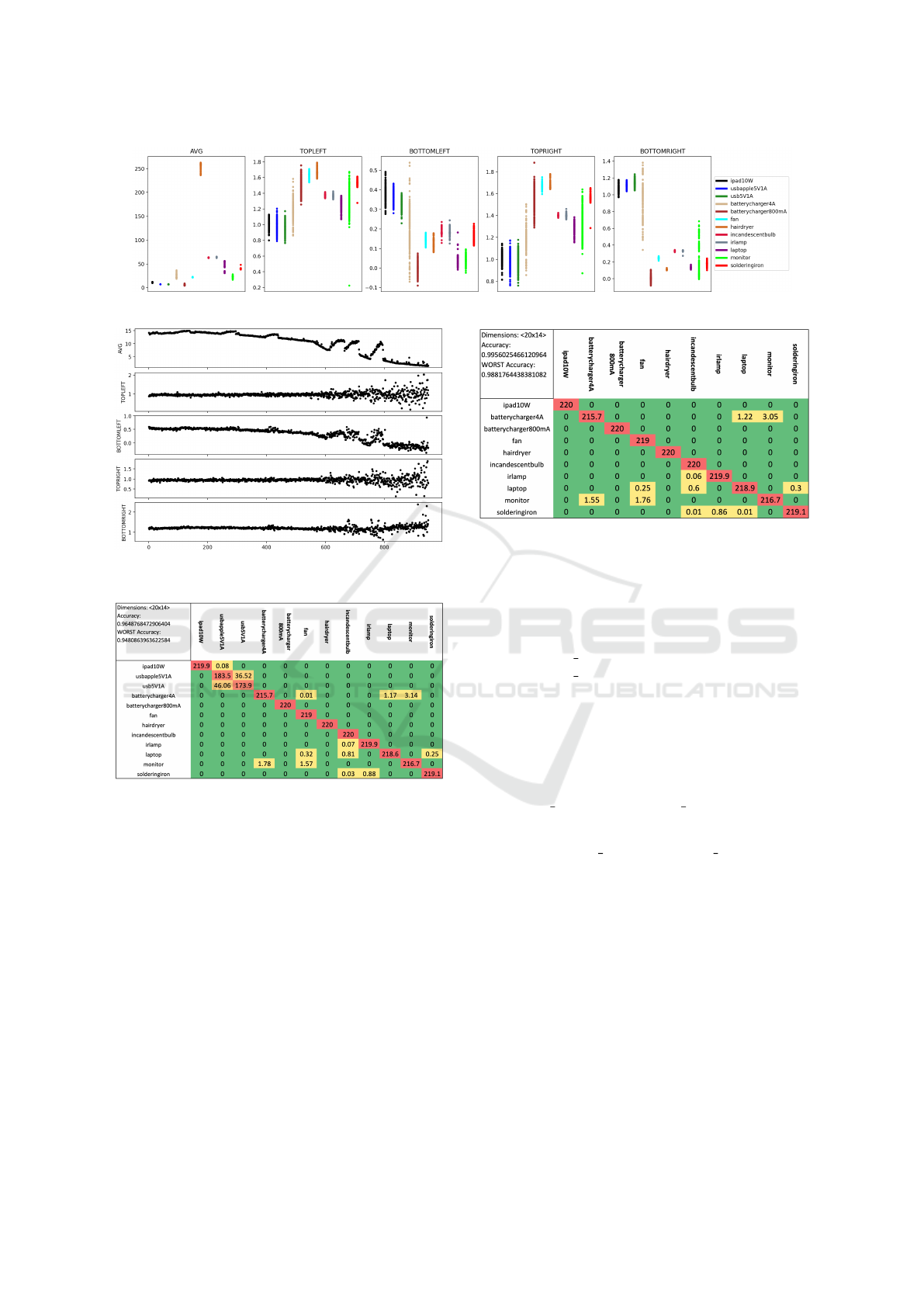
Figure 3: Five of the feature values plotted for the ﬁrst 250 measurements.

Figure 4: Five characteristics plotted for measurements

taken during the charging of the iPad.

Figure 5: Confusion matrix (average of 100 runs) of the

SVM classiﬁcation results. 30 samples from each class

were used for training.

5 MEASUREMENT PROFILES

The previous section showed that the SVM method

is accurate for classifying the measurement data col-

lected. The question is whether similar results can

be achieved with fewer data and if so, it also reduces

computational complexity. Less computational com-

plexity allows Edge Computing methods to be used

and may also make it possible to run the classiﬁcation

on the ESP32 microcontroller in the future.

The deﬁnition of measurement proﬁles is intro-

duced to modify the measurement parameters and en-

able the search for possible optimal choices. The

measurement proﬁle deﬁnes the parameters of the

Figure 6: Confusion matrix (average of 100 runs) of the

SVM classiﬁcation results. 30 samples from each class

were used for training. Only one USB class was used.

measurement. The measurement proﬁle consists of

the following:

• r - the number of different cutoff ratios

• percentage min - the minimal cutoff ratio

• percentage max - the maximum cutoff ratio

• h - the number of cycles the AC signal is cut for

each cutoff ratio

• d - the number of cycles where the AC signal is

not modiﬁed between measuring with two cutoff

ratios

The cutoff ratios are evenly spaced between

percentage min and percentage max. The measure-

ment proﬁles will be shown in the following form:

{< r, percentage min − percentage max >,h, d}

The number of cycles (one full period of the AC volt-

age signal - 20ms) required for one full measurement

with a measurement proﬁle can be calculated using

the following formula:

cycles

= h · r + d · (r − 1) (3)

Multiple submatrices can be extracted from orig-

inal measurements and used for classiﬁcation. These

submatrices extract the data that the measurement

proﬁle would have collected. (E.g.: if h = 6, then only

the ﬁrst six columns of the original matrices would

be considered.) Running the simulations for multiple

parameters shows an estimate of how accuracy would

change using different measurement proﬁles. Using

SMARTGREENS 2022 - 11th International Conference on Smart Cities and Green ICT Systems

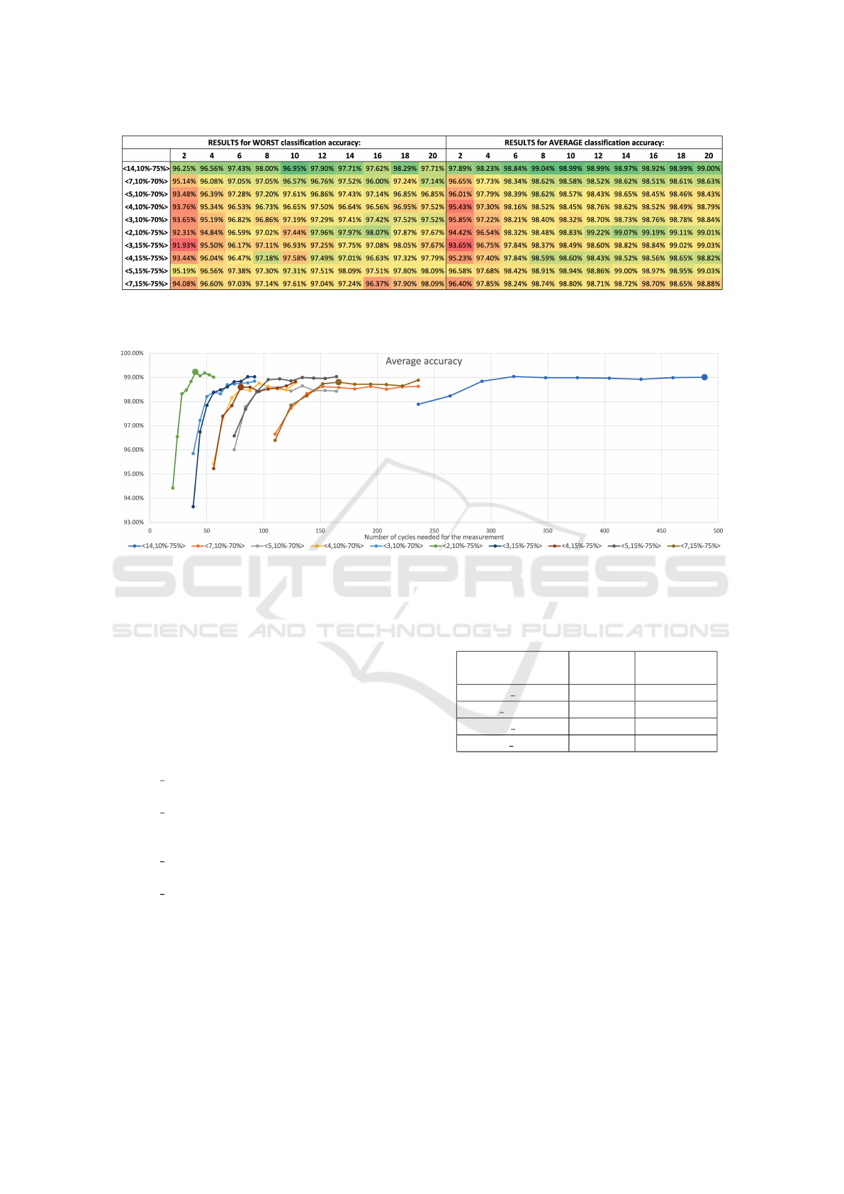
Figure 7: Simulations ran on an early version of the created dataset, 100 samples from each class, 30 used for training. The

vertical axis shows the cutoff ratios, and the horizontal shows the number of AC cycles for each cutoff ratio. Each simulation

was run 100 times, and the worst and average accuracy values were shown.

Figure 8: Average simulation results plotted for each cutoff ratio set. The bigger markers show the measurement proﬁles

chosen. The horizontal axis shows the number of cycles each measurement would take assuming d = 16.

different cutoff ratio numbers between 2 and 14 and

different h values between 2 and 20, the accuracy re-

sults can be seen in Figure 7.

Then we can choose measurement proﬁles to use

for actual measurement collection. In the plots of the

results for each measurement ratio set (Figure 8), it

can be seen that by increasing h, the change in ac-

curacy slows down, and only the measurement time

increases. Based on this data, the following measure-

ment proﬁles were selected:

• TEST ORIG : {< 14, 10% − 75% >,h = 20, d =

16} Measurement time: 488 AC cycles (9.76s)

• TEST HALVED : {< 7, 15% − 75% >, h =

10, d = 8} Measurement time: 118 AC cycles

(2.36s)

• TEST TINY : {< 2, 10% −75% >, h = 12, d = 4}

Measurement time: 28 AC cycles (0.56s)

• TEST FOUR : {< 4, 15% − 75% >, h = 8, d = 4}

Measurement time: 44 AC cycles (0.88s)

In Figure8, the selected measurement proﬁles are

shown with a bigger maker.

The software of the microcontroller was also mod-

iﬁed to allow measurements with measurement pro-

ﬁles. Data was collected for the same devices listed

in Section 3.3. For each measurement proﬁle, at least

Table 1: SVM Classiﬁcation results for each measurement

proﬁle. Each classiﬁcation was run 100 times, the average

accuracy values are shown.

Measurement

proﬁle

All USB

classes

One USB

class (iPad)

TEST ORIG 96.49% 99.56%

TEST HALVED 93.36% 98.74%

TEST TINY 91.89% 97.40%

TEST FOUR 94.42% 99.35%

250 measurements were taken per class.

The results of the SVM classiﬁcation with mea-

surement proﬁles can be seen in Figures 9 (with sep-

arate USB classes) and 10 (one usb class - iPad). It

can be seen that with the reduced amount of data col-

lected, the classiﬁcation accuracy decreases, but the

average accuracy values are still over 91%. Table 1

summarizes the classiﬁcation accuracy results for all

measurement proﬁles.

A small training sample size (30) is enough to

achieve above 99% accuracy with the SVM classiﬁca-

tion method. This means that only a few minutes are

required to collect the necessary measurements and

proﬁle a device.

SP4LC: A Method for Recognizing Power Consumers in a Smart Plug

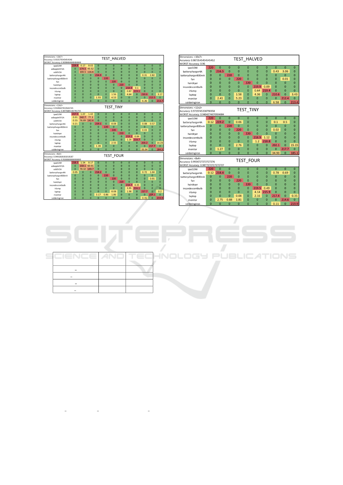
Figure 9: Confusion matrix (average of 100 runs) of the

SVM classiﬁcation results for the new measurement pro-

ﬁles. 30 samples from each class were used for training.

The column class labels are the same as in Figure 5.

Table 2: FC NN Classiﬁcation results for each measurement

proﬁle. Each classiﬁcation was run 100 times, one USB

class was used.

Measurement

proﬁle

Average

accuracy

Worst

accuracy

TEST ORIG 99.51% 98.53%

TEST HALVED 98.52% 94.07%

TEST TINY 97.88% 96.20%

TEST FOUR 98.50% 97.20%

6 DATA CLASSIFICATION WITH

NEURAL NETWORKS

The data were also classiﬁed with a simple, Fully

Connected Neural Network. The input layer used the

ten features chosen in Section 4, and two hidden lay-

ers of sizes 10 and 6 were used. The activation func-

tion was ReLU. The result can be seen in Figure 11,

and the results are summarized in Table 2.

6.1 Classiﬁcation with CNN

Convolutional Neural Networks are popular solu-

tions in image processing tasks. As in the cases of

the TEST ORIG, TEST HALVED, and TEST FOUR

Figure 10: Confusion matrix (average of 100 runs) of the

SVM classiﬁcation results for the new measurement pro-

ﬁles. 30 samples from each class were used for training.

Only one USB class was used. The column class labels are

the same as in Figure 6.

measurement proﬁle matrices, we can interpret the

task at hand as an image processing task with a low-

resolution input image. Using only the power ma-

trix, the network could not distinguish between the

incandescent light bulb and the infrared lamp. As

it turns out, the infrared lamp used for the measure-

ments is also an incandescent bulb emitting infrared

radiation, so we expect them to have similar char-

acteristics. This inability to distinguish between the

same kind of devices shows the CNN’s capability to

extract generalized features and shows the network’s

deeper understanding of the connected load.

The CNN consisted of two convolutional lay-

ers with (3 × 3) kernels. The ﬁrst used ReLU and

padding, while the second did not use padding and

used softmax as the activation function. We were

using softmax provided normalization before the FC

layers. The ﬁrst convolutional layer extracted 48 fea-

tures, while the second extracted 64 features. After

ﬂattening the layers, two hidden, fully connected lay-

ers with ReLU activation function were used (48 and

64 neurons) before the ﬁnal layer with softmax acti-

vation. The results of the classiﬁcation can be seen

in Figure 12. By using the Power, the Voltage (di-

vided by 230), and the Current matrices, 50 samples

for each class in the training set are enough to achieve

SMARTGREENS 2022 - 11th International Conference on Smart Cities and Green ICT Systems

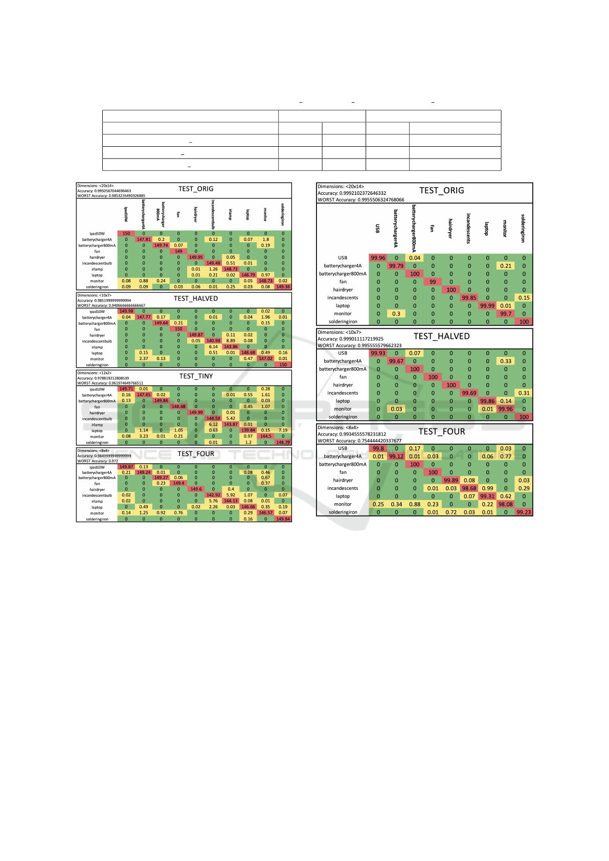
Table 3: CNN Classiﬁcation results for the TEST ORIG, TEST HALVED and TEST FOUR proﬁles.

Used data — Training samples per class Power — 150 Power, Voltage, Current — 50

Accuracy avg worst avg worst

TEST ORIG 99.92% 99.56% 99.84% 99.50%

TEST HALVED 99.90% 99.56% 99.86% 99.44%

TEST FOUR 99.35% 75.44% 98.81% 82.17%

Figure 11: Confusion matrix (average of 100 runs) of the

FC NN classiﬁcation results. 100 samples from each class

were used for training, 150 for testing. One USB class was

used.

the same accurate results. The results are shown in

Figure 13. Table 3 summarizes the results.

7 CONCLUSION

We have presented a solution to the fast classiﬁcation

of electric loads. The measurement time can be as

low as 0.56s, while a complete measurement takes

less than 10 seconds. We proposed different clas-

siﬁcation methods suited for different applications.

While deep networks such as CNN can provide high

(99.92% average) accuracy rate and better generaliza-

Figure 12: Confusion matrix (average of 100 runs) of the

CNN classiﬁcation results. A common USB class was used

for the three USB adapters, and the incandescent light bulb

and the infrared lamp were merged to one class (incandes-

cents). 150 samples from each class were used for training

the model, 100 were used for testing.

tion, the computational requirements are much higher.

For edge computing solutions, traditional FC NN and

SVM provide a better solution to achieve similar re-

sults with less computational resources. If the data

collection is the bottleneck, then SVM is the best op-

tion as a small dataset is enough thanks to the care-

fully selected features used for the input of the SVM

classiﬁcation. As SVM requires the least amount of

computational power from the methods presented, it

is ideal for on-device classiﬁcation. Classiﬁcation on

the microcontroller of the measurement prototype de-

vice is one area considered for future research related

SP4LC: A Method for Recognizing Power Consumers in a Smart Plug

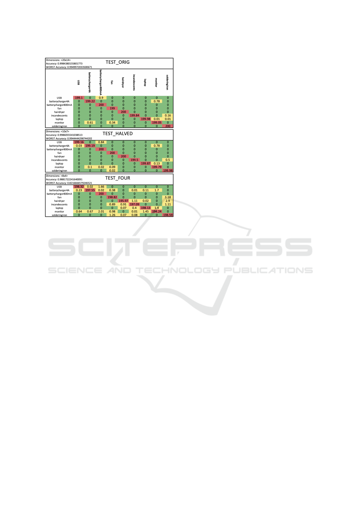
Figure 13: Confusion matrix (average of 100 runs) of the

CNN classiﬁcation results using the Power, Current, and

Voltage(divided by 230) matrices. A common USB class

was used for the three USB adapters, and the incandescent

light bulb and the infrared lamp were merged into one class

(incandescents). Fifty samples from each class were used

for training the model, 200 were used for testing.

to this topic.

We have also introduced measurement proﬁles

that show that even less data is enough to classify the

connected load accurately. A reduction of the amount

of collected data also reduces the computational re-

quirements of the classiﬁcation. Based on the require-

ments of the classiﬁcation system, the data collection

can be optimized with the help of measurement pro-

ﬁles to achieve faster device labeling and data pro-

cessing while decreasing accuracy only by a small

amount.

7.1 Future Work

With the method presented, we have shown that with

only 30 training samples, SVM classiﬁcation could

achieve an average of 99.56% accuracy rate. This

means that even with the longest test proﬁle, the train-

ing data collection requires less than 6 minutes of

measurement per electric load. The CNN approach

shows that the network can understand the type of

features and can generalize, so similar types of de-

vices (like USB chargers) will be accurately classi-

ﬁed; however, the current system cannot detect new

types of electric loads that were not measured previ-

ously. Detecting a previously unknown device as un-

known is a complex task. In future work, we intend to

examine Open Set classiﬁcation methods for detect-

ing previously unseen devices. A smart plug system

with Open Set classiﬁcation methods could automat-

ically trigger the training data collection for a previ-

ously unseen load. User interaction would only be

needed for providing a label for the device.

The other area considered for future work is the

classiﬁcation on the microcontroller. The methods

presented may enable the classiﬁcation of the con-

nected load on the ESP32 microcontroller inside the

prototype device. With the WiFi capabilities of the

microcontroller, a Wireless Sensor Network could be

built. As the dimmer used in the prototype device can

cut the connected load’s power supply, the prototype

is capable of not only measuring but also controlling

the load, so no hardware modiﬁcations would be re-

quired for a smart plug system.

ACKNOWLEDGEMENTS

Supported by the

UNKP-20-1 and

UNKP-21-1 new

national excellence program of the ministry for inno-

vation and technology from the source of the national

research, development and innovation fund.

REFERENCES

da S. Veloso, A. F., de Oliveira, R. G., Rodrigues, A. A.,

Rabelo, R. A. L., and Rodrigues, J. J. P. C. (2019).

Cognitive smart plugs for signature identiﬁcation of

residential home appliance load using machine learn-

ing: From theory to practice. In 2019 IEEE Inter-

national Conference on Communications Workshops

(ICC Workshops), pages 1–6.

Du, L., He, D., Harley, R. G., and Habetler, T. G. (2016).

Electric load classiﬁcation by binary voltage–current

trajectory mapping. IEEE Transactions on Smart

Grid, 7(1):358–365.

Gomes, L., Sousa, F., Pinto, T., and Vale, Z. (2019). A

residential house comparative case study using market

available smart plugs and enaplugs with shared knowl-

edge. Energies, 12:1647.

Gomes, L., Sousa, F., and Vale, Z. (2018). An intelligent

smart plug with shared knowledge capabilities. Sen-

sors, 18(11):3961.

Jaradat, M., Jarrah, M., Jararweh, Y., Al-Ayyoub, M., and

Bousselham, A. (2014). Integration of renewable

energy in demand-side management for home appli-

ances. In 2014 International Renewable and Sustain-

able Energy Conference (IRSEC), pages 571–576.

SMARTGREENS 2022 - 11th International Conference on Smart Cities and Green ICT Systems

Petrovi

c, T. and Morikawa, H. (2017). Active sensing ap-

proach to electrical load classiﬁcation by smart plug.

In 2017 IEEE Power Energy Society Innovative Smart

Grid Technologies Conference (ISGT), pages 1–5.

Ridi, A., Gisler, C., and Hennebert, J. (2014). A survey

on intrusive load monitoring for appliance recogni-

tion. In 2014 22nd International Conference on Pat-

tern Recognition, pages 3702–3707.

SP4LC: A Method for Recognizing Power Consumers in a Smart Plug