Using Machine Learning and Finite Element Modelling to Develop a

Formula to Determine the Deflection of Horizontally Curved Steel

I-beams

Elvis M. Ababu

, George Markou

and Nikolaos Bakas

Department of Civil Engineering, University of Pretoria, Lynnwood Road, Pretoria, South Africa

Department of RnD, RDC Informatics, Athens, Greece

Keywords: Curved Beams, Machine Learning, Steel, Finite Element Method, Design.

Abstract: The use of curved I-beams has been increasing throughout the years as the steel forming industry continues

to advance. However, there are often design limitations on such structures due to the lack of recommendations

and design code formulae for the estimation of the expected deflection of these structures. This is attributed

to the lack of understanding of the behaviour of curved I-beams that exhibit extreme torsion and bending.

Thus, currently, there are no formulae readily available for practising engineers to use to estimate the

deflection of curved beams. Since the design of light steel structures is often governed by serviceability

considerations, this paper aims to analyse the properties of curved steel I-beams and their impact on deflection

as well as develop an accurate formula that will be able to predict the expected deflection of these beams. By

using a combination of an experimentally validated finite element modelling approach and machine learning.

Numerous formulae are developed and tested for the needs of this research work. The final proposed formula,

which is the first of its kind, was found to have an average error of 4.11% in estimating the midspan deflection

on the test dataset.

1 INTRODUCTION

A beam is a structural element that has been studied

extensively for numerous years and is used widely,

not only in the field of civil engineering but

mechanical engineering as well. The use of curved

steel I-beams have been increasing steadily

throughout the years due to the aesthetically pleasing

designs that they produce in buildings as well as for

industrial applications. Horizontally curved steel I-

sections can be found in various applications ranging

from girders in modern highway bridges, interchange

facilities as well as in industrial buildings where they

are used as crawl beams. Due to advancements in

steel forming technology, almost any section can be

curved with minimum limitations that relate to the

beam’s section size or length. Numerous studies have

been conducted in efforts to understand the behaviour

of curved beams based on different materials as

discussed in (Al-Hassaini, 1962), (McManus et al.,

1969), (Hsu et al., 1978, Mansur and Rangan, 1981),

(Al-Hashimy and Eng, 2005), (Chavel, 2008) and

(Lee et al., 2017). It is widely known that, unlike

straight beams, horizontally curved beams subject to

gravity loads experience a complex system of

combined effects, namely, shear, flexure and torsion.

This loading effect causes a complex structural

response such as warping due to non-uniform torsion.

The study of curved girders began with Umanskii

(1948) who obtained solutions for curved beams

based on several loading conditions by assuming

initial parameters in the solution procedure (Liew et

al., 1995). Numerous other studies and experiments

have been conducted from the 1960s to the present

day, however, these studies mainly focused on the

ultimate limit states of the beam and not on the

serviceability limit states. Those that did focus on

serviceability limit states design, did not analyse the

effect various parameters have on deflection, whereas

those that did analyse the effect on deflection did not

determine an appropriate formula without using

Castigliano’s second theorem. Currently, most design

codes (SANS, AISC, Eurocode 3, etc.) do not have a

section detailing deflection estimation of curved steel

I-beams. AISC however does state that the usage of

finite element modelling (FEM) is appropriate when

958

Ababu, E., Markou, G. and Bakas, N.

Using Machine Learning and Finite Element Modelling to Develop a Formula to Determine the Deﬂection of Horizontally Curved Steel I-beams.

DOI: 10.5220/0010982400003116

In Proceedings of the 14th International Conference on Agents and Artiﬁcial Intelligence (ICAART 2022) - Volume 3, pages 958-963

ISBN: 978-989-758-547-0; ISSN: 2184-433X

deflection results are of importance (Dowsell, 2018).

The issue arises when Engineers conduct a linear

static analysis on the structure as a whole and check

deflections in that manner. The issue with that

approach is that curved beams experience large

deflections, which leads to nonlinear strain-

displacement and curvature-slope relations, a

phenomenon that necessitates accounting for

geometric nonlinearities. Another approach would be

to use Castigliano’s second theorem which is

numerically tedious (Dahlberg, 2004). Nevertheless,

researchers have attempted to provide a formula for

deflection of curved steel I-beams based on

Castigliano’s second theorem, however, this formula

is often not readily available to practising engineers

and is only applicable for specific support and loading

conditions.

This research work attempts to derive an easy to

use formula to determine the midspan deflection of

real cantilever types of curved steel I-beams with

loads applied only at the midspan. A machine

learning algorithm that uses nonlinear regression is

implemented herein to create a closed-form equation

based on midspan deflection results, a dataset

developed through the use of Reconan FEA (2020)

(Mourlas and Markou, 2020). Prior to the

development of the models that were used to train the

machine learning algorithm, the software was

validated through the use of experimental results

found in (Shanmugam et al., 1995). It should be noted

herein that the final curved beam properties must be

used because typically beams are curved through a

cold process known as pyramid roll bending which

alters the material properties of the steel (Dowsell,

2018). After developing different formulae through

training the machine learning algorithm on the

developed dataset, an investigation on the prediction

ability of each formula was performed. The factors

considered for developing the formulae that foresaw

different numbers of features, were: section area (A),

curved length of the beam (L), the radius of the beam

(R), yielding strength (f

), Young’s modulus (E).

2 MACHINE LEARNING

ALGORITHMS

Machine learning has grown in popularity in recent

years in numerous scientific fields, including civil

engineering. The power of machine learning

algorithms is that even though complex nonlinear

models seem to present no correlation in small sample

spaces, by considering a large enough sample a

pattern emerges, which can then be exploited to

generate a formula to predict out-of-sample data.

Various machine learning and artificial intelligence

methods are applied for engineering problems such as

Random Forests, Gradient Boosting and Artificial

Neural Networks, amongst others. The issue with

such models is that their results often cannot be

interpreted in practical cases unless integrated into

some software. In this work, a higher-order nonlinear

regression modelling framework was utilized

(Gravett et al., 2021) due to its ability to provide an

explicit closed-form formula. The model is based on

the creation of nonlinear terms based on the

independent variables up to the third degree. The

algorithm automatically selects the nonlinear features

which would correspond to the minimum error. The

algorithm found in Table 1 represents the procedure

that would lead to the development of the desired

formula:

Table 1: Higher-Order Nonlinear Regression Algorithm

(Gravett et al., 2021).

Input: XX (matrix of Independent Variables), YY

(Vector of Dependent Variable), nlf (number

of nonlinear features to be ke

t in the model

)

Output: Prediction Formulae

1. Create all nonlinear features

(

anl

)

2. For i from 1 to nlf, do:

3. For

from 1 to anl

, do:

4. Add

feature to the model

5. Calculate Prediction Error, MAPE

6. END

7. Keep in the model the j

feature

which yields the minimum

rediction erro

8. END

Return: Prediction Formula

3 NUMERICAL CAMPAIGN

This section presents the procedure adopted to

generate the dataset that will be presented thereafter.

Initially, a mesh sensitivity analysis was performed to

determine the optimum mesh size, where the ability

of Reconan FEA (2020) to calculate the mechanical

response of these types of beams is investigated.

Then, beams with varying geometrical and material

properties were developed and analysed for

constructing the dataset that was used to train the

machine-learning algorithm presented in the previous

section. Finally, the predictive models that were

developed as closed-form formulae, were

parametrically tested on additional data to determine

Using Machine Learning and Finite Element Modelling to Develop a Formula to Determine the Deﬂection of Horizontally Curved Steel

I-beams

959

their ability to predict the deformation at the midspan

of the curved steel I-beams.

3.1 Mesh Sensitivity and Validation

Analysis

A mesh sensitivity analysis was conducted to

determine a mesh size that derives the optimal results

of an experiment found in Shanmugam et al. (1995).

It was decided to compare 8 noded and 20 noded

hexahedral elements with element sizes of 20, 30, 50,

and 100 mm hexahedral element sizes for this

investigation. The developed models can be seen in

Figure 1. The numerically obtained curves were

compared with the experimental curve found in

Shanmugam et al. (1995).

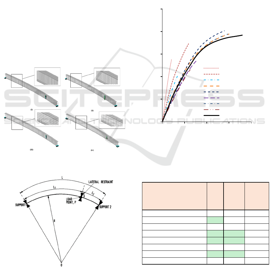
Figure 2 shows the experimental setup of the

beam tested by Shanmugam et al. (1995) and

investigated numerically herein. As it can be seen, the

curved length of the beam (L) is 5 m, the point of load

application (L

) 3.8 m from the left support and the

radius (R) is 20 m.

Figure 1: Mesh sensitivity analysis models with mesh sizes,

(i) 20mm, (ii) 30mm, (iii) 50mm, (iv) 100mm.

Figure 2: Experimental setup (Shanmugam et al., 1995).

Nonlinear analyses were performed using Reconan

FEA (2020) that foresaw 100 load increments and an

energy convergence tolerance of 10

-5

. It is important

to note that only material nonlinearities were

accounted for in the developed models through

adopting the von Mises yielding criterion. The final

results of the mesh sensitivity analysis can be seen in

Figure 3 and Table 2. It is easy to depict that most

beams managed to come close to the ultimate load as

found in the experimental data, however, the beams

with the coarse mesh failed to accurately model the

ductility of the steel and in general reproduce the

overall mechanical response of the curved beam.

Figure 3: Graphically comparing load-deflection results of

various mesh sizes against experimental data.

Table 2: Numerical comparison of the various mesh sizes

against experimental data.

The 50 mm, 20-noded isoparametric hexahedral

finite elements derived the best results with a 1.5%

100

150

200

250

0 20406080

Load (kN)

Deflection (mm)

8 noded with 0.1m elements

20 noded with 0.1m elements

8 noded with 0.05m elements

20 noded with 0.05m elements

8 noded with 0.03m elements

20 noded with 0.03m elements

8 noded with 0.02m elements

20 noded with 0.02m elements

Experimental data

Model

/Δ

Analysis

time

(hh:mm:ss)

8 noded with 0.1m elements 1.376 8.588 00:21.9

20 noded with 0.1m elements 1.108 3.049 01:22.6

8 noded with 0.05m elements 1.813 5.040 01:04.5

20 noded with 0.05m elements 0.985 1.199 05:16.3

8 noded with 0.03m elements 0.950 1.288 06:17.0

20 noded with 0.03m elements 1.425 2.371 15:12.3

8 noded with 0.02m elements 0.985 1.218 16:20.9

20 noded with 0.02m elements 1.662 2.874 03:06:05

ICAART 2022 - 14th International Conference on Agents and Artiﬁcial Intelligence

960

error in predicting the ultimate failure load, less than

20% error for capturing the max deflection at failure

and 6.33% error in estimating deflection at 50% of the

total load. It is evident that this experiment did not

develop any local or global buckling prior to ultimate

failure, thus the nonlinear detailed model was able to

capture the overall mechanical response with

acceptable accuracy.

3.2 Finite Element Models

Figure 4 shows the 20-noded hexahedral mesh of one

of the beams that were analysed in this paper for

different material properties, while other beams were

developed with different geometric properties. It was

chosen to place a fixed support on the left side of the

beam and a roller support on the right side of the beam

which closely represents the boundary conditions as

experienced by crawl beams in industrial buildings.

The load was placed at the centre span of the beam

and were divided into 100 load increments to

accurately determine the midspan deflection. The

loads were placed on the web of the member to avoid

local failure of the flange.

Numerous beams were created to make sure the

formula encompasses a large variety of parameters.

The parameters considered in this study included the

curved length of the beam (L), the radius of the curve

(R), the Young’s modulus of steel (E), and the section

sizes. It is also noted that specific combinations of

these input parameters are of significance in

analysing curved beams, specifically, the R/L ratio

which is an indication of the amount of curvature a

beam experiences. This shall be considered in the

sensitivity analysis later but will lead to

complications when developing the formula. A total

of 270 beams were initially created, where, 3 I-beam

sections were considered, namely a 305x165x46UB,

533x210x82UB and a 203x133x25UB. These beam

sections represent the extreme ends of I-beam

sections that are commercially available in South

Africa as well as an intermediate beam size. All

beams were analysed until failure, where the ultimate

load was recorded. Various points along the elastic

load-deflection diagrams were considered which lead

to a total number of 1890 unique data points to train

the machine learning algorithm. To ensure that the

points were on the elastic region, the points that were

selected foresaw a maximum of 50% load level of the

maximum load level as computed from the analysis.

A statistical summary of the various properties

can be seen in Table 3. Where A is the section area in

and I

is the second moment of area of the cross-

section about the x-axis in mm

. A large number of

radii were considered as this was hypothesised to be

the parameter to have a significant impact on the

deflection.

Figure 4: General beam undeformed mesh.

Table 3: Statistical summary of independent variables.

Metric

(mm

)

(mm

)

(m)

(GPa)

mean 2.02x10

6.58x10

5.02 58.99 205.10

std 1.99 x10

3.02x10

1.64 47.55 8.38

median 9.93 x10

5.88x10

5.00 60.00 205.10

min 2.35 x10

3.22x10

3.00 3.50 194.85

max 4.75 x10

1.05x10

7 140.00 215.36

Figure 5: General beam deformed shape and Von Mises

stress contour.

4 RESULTS AND VALIDATION

Figure 5 shows the general deflected shape that the

beam experienced as well as the von Mises stresses

developed throughout the beam at 50% of the

ultimate load. It is easy to observe that torsion

dominates the beam while controlling the type of

failure. This was expected due to the eccentricity of

the load and shows that the mechanical behaviour of

the beam is as expected. The maximum stress

experienced was close to the pin-like support, where

the failure occurred at the bottom flange of the section

due to excessive stresses. This was a mechanical

response that was noted in all understudy curved steel

I-beams. The beams that had a low R/L ratio (beams

with lower curvature) failed close to the pin-like

Using Machine Learning and Finite Element Modelling to Develop a Formula to Determine the Deﬂection of Horizontally Curved Steel

I-beams

961

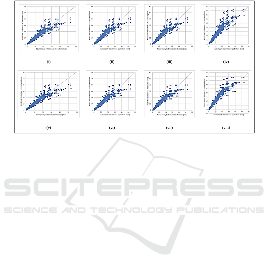
Figure 6: Correlation between numerically determined deflection and (i) 40 term, (ii) 25 term, (iii) 20 term, (iv) 15 term, (v)

13 term, (vi) 10 term, (vii) 7 term and (viii) 5 term formulae.

support, while failure occurred at the web and not

within the flange. It should, however, be noted that

failure analysis was not the subject of this research

work but rather, the deflection experienced during the

loading within the elastic region, which is what

interests Civil Engineering designers.

Once the models were analysed, a numerical

database was created that contained the parameters of

each beam and the respective midspan deflections

(one row per deflection point). This numerical

database was then used to train the machine learning

algorithm, which was able to provide formulae as

well as other descriptive statistics about the training

and testing process (sensitivity analysis that will be

presented in an extended version of this manuscript).

When generating the formulae, as was seen in the

machine learning section of this manuscript, the beam

features are considered as input parameters. A range of

5 to 40 features were considered when training the

formulae and the various results were compared to

determine the most accurate formula in terms of

predictability. Figure 6 shows the graphs comparing

the generated formulae to the numerically computed

deflection. As can be seen, there is a strong correlation

between the numerically determined deflections and

the deflections predicted by the various formulae.

In order to quantify the accuracy of the proposed

formula on the training and test set, several error

metrics were used, namely, the correlation coefficient

), alpha metric (α), the root mean square error

(RMSE), the mean absolute error (MAE), the mean

absolute percentage error (MAPE), the max absolute

percentage error (MAXPE), and the quotient error

(SR).

It was seen that as the number of features

decreases, the error increases, a numerical response

that is in line with the finding reported by Gravett et

al. (2021). Some error metrics, such as the r

, barely

change as the number of features changes (the r

error

was seen to be approximately 0.95 regardless of the

number of features), however, other metrics such as

MAXPE change drastically as the number of features

increase (MAXPE ranged from 1.9607 when 5

features were used to 0.7850 when 40 features were

used). This shows the importance of considering

numerous error metrics in determining the optimum

formula that will show advanced predictive

capabilities. It must be noted here that the dataset was

divided into 85% and 15%, training and testing data,

respectively.

4.1 Validation

After training and testing the numerous formulae that

were discussed in the previous section, the proposed

formulae were then further validated by creating an

out of sample model and estimating the midspan

deflection. The beam considered was a 305x127x42

UB with a curved length of 5 m and a radius of 20 m.

The Young’s modulus of the beam was also varied

(205.1 GPa, 200 GPa and 210 GPa). Various ultimate

load percentages were also considered in this

validation process, where a total of 15 new data points

were developed for the needs of this investigation. It

ICAART 2022 - 14th International Conference on Agents and Artiﬁcial Intelligence

962

was found that the function that consisted of 10

features derived the lowest average error, of only

4.11% in estimating the deflection of 15 out-of-

sample data points, while the model with 40 features

resulted in the largest error of 13.05%. This is a

numerical phenomenon that is usually attributed to

overfitting during the training and testing procedure.

The proposed formula used to estimate the

deflections that consisted of 10 terms can be seen in

Equation 1. The various independent variables are E

which is the Young’s modulus in GPa, L is the curved

length of the beam in metres, A is the section area in

, f

is the yielding stress, I

is the second moment

of area about the strong axis in mm

and Q is the

percentage of ultimate loading applied on the beam as

a number (50% = 50). The resulting deflection from

the formula is in mm.

𝐷𝑒𝑓𝑙𝑒𝑐𝑡𝑖𝑜𝑛 = 1.08128 ∗ 10



∗ 𝑄 ∗ 𝐿 − 8.41124

∗10



∗ 𝑄 ∗ 𝐿 ∗ 𝐴 − 9.81969

∗10



∗ 𝑄 ∗ 𝐸 ∗ 𝑅 + 1.82604

∗10



∗ 𝑄 ∗ 𝑅 ∗ 𝑅 − 2.71029

∗10



∗ 𝑄 ∗ 𝑅 ∗ 𝐿 + 6.22991

∗10



∗ 𝑄 ∗ 𝐿 ∗ 𝐿 + 2.55963

∗10



∗ 𝑄 ∗ 𝐿 ∗ 𝐼𝑥𝑥 + 2.99150

∗10



∗ 𝑄 ∗ 𝑄 ∗ 𝑓𝑦 + 4.19580

∗10



∗ 𝑄 ∗ 𝑓𝑦 ∗ 𝑓𝑦 − 1.07754

∗10



∗ 𝑄 ∗ 𝐸 ∗ 𝐿 − 8.95792

∗10



(1)

5 CONCLUSIONS

A formula was successfully developed for the

prediction of the deflection of curved steel I-beams.

When comparing the proposed formula with the out-

of-sample data, it was found that the formula

containing 10 features was the most accurate, having

an average error of 4.11%, while the formula with 40

features was the least accurate having an error of

13.05%. The lack of accuracy in the 40 feature

equation was attributed to an over-fitting

phenomenon but can also be attributed to another

phenomenon known as the “interaction effect”, which

can greatly increase the effect of the independent

variables on the dependent variable.

Based on the parametric and sensitivity

investigation, it was concluded that the variables with

the largest impact on deflection are the curved length

and radius of the beams. Due to the page limitations

of this manuscript, the results of the in-depth

sensitivity analysis could not be shared, however,

these will be published at a later stage. Even though

the results of this study are positive seeing as very low

error metrics were observed, the study has to be

expanded in the future by developing additional

models with a larger spectrum in terms of geometries.

Various boundary conditions, as well as different

yield strengths of steel, will also be considered.

Experimental curved steel I-beams will also be tested

to validate the proposed formula developed in this

study. Future research work will foresee the

development of similar formulae on curved concrete

beams. Finally, the long-run objective is to develop

machine learning models that will be able to evaluate

the response of full scale-structures

REFERENCES

Al-hashimy, M. A. & Eng, P. Load distribution factors for

curved concrete slab-on-steel I-girder bridges. Masters

Abstracts International, 2005.

Al-hassaini, M. M. F. 1962. Graphs and tables for the

analysis and design of curved concrete beams. Virginia

Tech.

Chavel, b. W. 2008. Construction and detailing methods of

horizontally curved steel I-girder bridges. University of

Pittsburgh.

Dahlberg, T. 2004. Procedure to calculate deflections of

curved beams. International journal of engineering

education, 20, 503-513.

Dowsell, B. 2018. Design Guide 33: Curved Member Design,,

American Institute of Steel Construction,.

Gravett, D. Z., Mourlas, C., Taljaard, V.-L., Bakas, N.,

Markou, G. & Papadrakakis, M. 2021. New fundamental

period formulae for soil-reinforced concrete structures

interaction using machine learning algorithms and ANNs.

Soil Dynamics and Earthquake Engineering, 144,

106656.

Hsu, T. T., Inan, M. & Fonticiella, L. Behavior of reinforced

concrete horizontally curved beams. Journal Proceedings,

1978. 112-123.

Lee, K., Davidson, J. S., Choi, J. & Kang, Y. 2017. Ultimate

strength of horizontally curved steel I-girders with equal

end moments. Engineering Structures, 153, 17-31.

Liew, J. R., Thevendran, V., Shanmugam, N. & Tan, L. 1995.

Behaviour and design of horizontally curved steel beams.

Journal of Constructional Steel Research, 32, 37-67.

Mansur, M. A. & Rangan, B. V. Study of design methods for

reinforced concrete curved beams. Journal Proceedings,

1981. 226-254.

Mcmanus, P. F., Nasir, G. A. & Culver, C. G. 1969.

Horizontally curved girders-state of the art. Journal of the

Structural Division, 95, 853-870.

Mourlas, C. & Markou, G. 2020. ReConAn v2.00 Finite

Element Analysis Software User's Manual.

Reconan FEA v2.00, User’s Manual. 2020.

https://www.researchgate.net/publication/342361609_ReCo

nAn_v200_Finite_Element_Analysis_Software_User's_

Manual

Shanmugam, N., Thevendran, V., Liew, J. R. & Tan, L. 1995.

Experimental study on steel beams curved in plan.

Journal of Structural Engineering, 121, 249-259.

Umanskii, A. 1948. Spatial structures. Moscow (in Russian).

Using Machine Learning and Finite Element Modelling to Develop a Formula to Determine the Deﬂection of Horizontally Curved Steel

I-beams

963