On Conﬁguring Directional Transmission for Path Exposure Reliability

in Energy Harvesting Wireless Sensor Networks

Abdulsalam Basabaa and Ehab S. Elmallah

Department of Computing Science, University of Alberta, 8900 114 St NW, Edmonton, Canada

Keywords:

Wireless Sensor Networks (WSNs), Energy Harvesting Wireless Sensor Networks (EH-WSNs), Path Expo-

sure Problem, Probabilistic Graph, Network Reliability, Directional Transmission.

Abstract:

In this paper, we consider a path exposure problem in energy harvesting wireless sensor networks (EH-WSNs)

where nodes are equipped with directional communication devices. Nodes harvest energy from ambient en-

vironment (e.g., solar power), and manage ﬂuctuations in their stored energy by adjusting some of their

directional transmission parameters. Using a probabilistic graph model we formalize a problem, denoted

DirEXPO-RU, that quantiﬁes the ability of a network to detect and report traversal along a given path as

probability representing the reliability of the network in performing the path monitoring task. A problem that

arises in managing the network resources to maximize this reliability measure is to adjust the transmission

beam width of each node, given that nodes beam centers are given as input. We develop a heuristic algorithm

to deal with the problem, and use the algorithm in a framework for computing lower bounds on the reliability

of the overall network. The obtained numerical results show improvement in the achieved network reliability.

1 INTRODUCTION

Research work on wireless sensor networks (WSNs)

where nodes are capable of directing their transmis-

sion (and/or reception) has been receiving attention

for a number of years now (see, e.g., the surveys

of (Amac Guvensan and Gokhan Yavuz, 2011; Tao

and Wu, 2015) for applications in area and barrier

coverage). In general, directional communication of-

fers improvement over omnidirectional transmission

in terms of achieving longer range (in a certain direc-

tion) for a given level of energy consumption.

Our interest in this paper is on investigating the

beneﬁts of using this mode of transmission in the class

of energy harvesting wireless sensor networks (EH-

WSNs) that is currently receiving signiﬁcant atten-

tion. In particular, we are interested in quantifying the

beneﬁts of directional transmission to achieve good

network performance while taking a complex network

reliability measure as our objective function. We pur-

sue this goal in the context of investigating a path ex-

posure reliability measure.

The path exposure problem is a well-known WSN

problem where we want to compute the probability of

detecting a moving target along a given path (over a

period of time) through a WSN ﬁeld. Early results

on the problem appears in (Megerian et al., 2002;

Clouqueur et al., 2003). In (Megerian et al., 2002),

e.g., the authors present a model that utilizes energy

sensed from a moving target over a period of time.

The model is then used to ﬁnd a path of minimal ex-

posure using a shortest path algorithm. In (Clouqueur

et al., 2003), the authors analyze target detection

probability using different data fusion models, and

present a method to minimize network deployment

cost while achieving desired exposure levels. Sub-

sequently, in (Liu et al., 2009), the authors formalize

a minimal path exposure problem for WSNs employ-

ing directional communication. They develop a di-

rectional sensing model used to deﬁne two weighted

graphs that are used to reduce the minimal path ex-

posure problem into two discrete geometry problems.

Their results include developing two approximation

algorithms to solve the problem.

Our work here on a path exposure problem builds

on the results obtained in (Elmorsy et al., 2013;

Basabaa and Elmallah, 2019; Basabaa and Elmallah,

2020). In (Elmorsy et al., 2013), the authors formal-

ize a path exposure problem, called EXPO, on con-

ventional WSNs for surveillance applications where

nodes are subject to communication and/or sensing

failure. In (Basabaa and Elmallah, 2019; Basabaa

and Elmallah, 2020), we consider a restricted version

of the DirEXPO-RU problem, called EXPO-RU. In

(Basabaa and Elmallah, 2019), the EXPO-RU prob-

lem is formalized and an efﬁcient algorithm is pre-

Basabaa, A. and Elmallah, E.

On Conﬁguring Directional Transmission for Path Exposure Reliability in Energy Harvesting Wireless Sensor Networks.

DOI: 10.5220/0010981600003118

In Proceedings of the 11th International Conference on Sensor Networks (SENSORNETS 2022), pages 60-70

ISBN: 978-989-758-551-7; ISSN: 2184-4380

Table 1: Overview of some related results.

Reference

Problem

Obtained results

Non-iterative

improvable

algorithms

Iterative

improvable

algorithms

Current paper

DirEXPO-RU

Conﬁguring node’s beam width

(Basabaa and Elmallah, 2021)

EXPO-RU

X X

(Basabaa and Elmallah, 2019)

EXPO-RU

X X

(Basabaa and Elmallah, 2020)

EXPO-RU

X X

(Elmorsy et al., 2013)

EXPO

X X

sented to compute lower bounds on the exact solution

of the EXPO-RU problem. In (Basabaa and Elmal-

lah, 2020), a dynamic programming approach is pre-

sented to compute bounds on exact solutions of the

EXPO-RU problem from certain network subgraphs.

The main focus of this paper is on developing ap-

proaches to conﬁgure the beam width for each node in

the network, so as to obtain good path exposure reli-

ability for the entire network, as described in the next

sections.

The rest of the paper is organized as follows: Sec-

tion 2 gives an overview of related work. The used

system model is presented in Section 3. Section 4

discusses problem formulation and conﬁguration ap-

proaches. Based on the proposed conﬁguration ap-

proaches, Section 5 presents an efﬁcient heuristic al-

gorithm to conﬁgure the transmission beams of nodes.

Section 6 explains a framework to compute bounds

for the DirEXPO-RU problem, and lastly the per-

formance of the proposed approaches is evaluated in

Section 7.

2 LITERATURE REVIEW

Our work here lies in the intersection of three main re-

search areas: the general area of EH-WSNs, research

speciﬁc to the use of directional communication in

WSNs, and research on developing reliability assess-

ment methods using probabilistic graph models. In

the following, we touch on each of the three areas.

2.1 Work on EH-WSNs

We refer the reader to the surveys in (Adu-Manu

et al., 2018; Sudevalayam and Kulkarni, 2011). Spe-

ciﬁc algorithmic contributions in the area include the

work of (Jakobsen et al., 2010; Peng and Low, 2013;

Mart

ınez et al., 2014; Peng et al., 2015; Li et al.,

2020). In (Jakobsen et al., 2010), the authors present

a distributed routing algorithm for EH-WSNs that

aims at dynamically ﬁnding sustainable routes to the

sink. In (Peng and Low, 2013), the authors present

an energy neutral WSN routing algorithm based on

the Directed Diffusion paradigm by adding an admis-

sion control step before a node can reinforce a ﬂow

that serves a particular interest. In (Mart

ınez et al.,

2014), the authors consider wastage of harvested en-

ergy when a node’s battery reaches its limit and can

not be charged. The authors formalize a route se-

lection problem that aims at reducing network wide

overcharging-wastage in each time slot of the net-

work’s operation. In (Peng et al., 2015), the au-

thors present an energy neutral clustering algorithm

for EH-WSNs that divides system’s time into time

slots. In each time slot, the network is partitioned into

a user-speciﬁed number of clusters and the data is col-

lected in each cluster. In (Li et al., 2020), the authors

propose a priority task scheduling algorithm for EH-

WSNs, where the transmission method and order of

collected data are determined according to task prior-

ity and node’s remaining energy.

2.2 Work on Directional

Communication in WSNs

Examples of work done in this area include the

work of (Duan et al., 2019) where the authors con-

sider data collection in a rechargeable sensor network

that is powered by directional wireless power trans-

fer (DWPT). The DWPT provides directional energy

beams using higher antenna gain for increasing en-

ergy efﬁciency. Also, the work of (Zhang et al., 2009;

Zhu et al., 2019), where the authors in (Zhang et al.,

2009) study a strong barrier coverage problem in di-

rectional sensor networks. They present an integer

linear programming model, and present two efﬁcient

algorithms to solve the problem. The authors in (Zhu

On Conﬁguring Directional Transmission for Path Exposure Reliability in Energy Harvesting Wireless Sensor Networks

et al., 2019) discuss the problem of deploying envi-

ronmental energy harvesting directional sensor net-

works with the minimum cost, where targets have dif-

ferent coverage requirements and the average energy

harvesting rate of each node should not be less than

its consumption rate. They formulate a mixed inte-

ger linear programming problem, and propose three

heuristics algorithms to solve the problem.

2.3 Work on WSNs Reliability for a

Path Exposure Problem

Here, we position the work done in this paper among

a few results that we have recently obtained on the

EXPO-RU problem. Table 1 gives an overview of the

results. In Table 1, the EXPO problem is the path

exposure reliability problem on conventional WSNs

where nodes are subject to failure (either in commu-

nication or sensing). Methods of assessing the net-

work reliability are classiﬁed as being either itera-

tively improvable or non-iteratively improvable. The

earlier type can achieve exact results if allowed to

work to completion. Else, they provide either a lower

bound (LB), or and upper bound (UB). In contrast,

the latter type produces a single bound (LB or UB)

on each input. Our work in this paper on conﬁgur-

ing beam width in directional transmission utilizes an

iteratively improvable LB algorithm to obtain numer-

ical results.

3 OVERVIEW OF SYSTEM

MODEL

In this section, we introduce the needed assumptions

and notations about the node model, the network

model, and the directional transmission model.

3.1 Node Operation Model

We assume that each node x in a given EH-WSN is

equipped with a directional communication device,

and an omnidirectional sensing device. Energy har-

vested at each node x ﬂuctuates over time. For the

purpose of simulating the network (e.g., to obtain

the probability distributions mentioned below), we as-

sume that time is divided into equal length slots.

Since wireless transmission is the most energy

consuming activity in many WSNs, we assume that

such ﬂuctuations affect the transmission range of a

node (but does not affect much its sensing range). An

energy management unit (EMU) in each node con-

trols a node’s state during any time slot. Our work

employs a multi-state node model for each node. In

its basic form, the model associates 3 states with each

non-sink node x, deﬁned as follows.

• If x’s stored energy level during a time slot lies

in some high range (say, e.g., [70%-100%]) of its

total energy storage capacity then the EMU puts x

in a full energy state where the node’s maximum

transmission range, denoted R

f ull

, is high.

• Else, if x’s stored energy level during a time slot is

in some lower range (say, e.g., [40%-70%]) of its

total energy storage capacity then the EMU puts x

in a reduced energy state where the node’s maxi-

mum transmission range, denoted R

red

, is lower.

• Else, if x’s stored energy level is lower than the

above, we consider the node to be in a failed state.

3.2 Network Reliability Model

Similar to our previous work in (Basabaa and Elmal-

lah, 2019), we adopt a network reliability model that

abstracts the above node dynamics over a long oper-

ation time by associating with each node x a prob-

ability distribution where for each possible state s ∈

{ f ull,reduced, f ail} we know the probability p

(x)

(also denoted p(x,s)) that node x is in state s (here,

f ail

(x) = 1 − p

f ull

(x) − p

red

(x)). In addition, we as-

sume that different nodes are assigned different states

independently of each other. Such an assumption is

common in the literature to simplify the analysis, and

also to take care of applications where different nodes

perform different tasks independent of each other.

In overall, an EH-WSN is modelled over a long

period of time by a probabilistic graph (G, p) where

G = (V ∪ {sink}, E) is a directed graph on a set V of

EH wireless nodes, a non-EH and fully operational

sink node, and a set E of directed communication

links (also referred to as directed edges or arcs). The

length of each arc (x,y) ∈ E emanating from a node

x depends on the energy state of x and also the direc-

tional transmission parameters associated with x, as

explained below. We note that G is a directed multi-

graph with parallel arcs. Parallel arcs from a node a

to a node b arise since if (a, b) exists when a is in the

full energy state then (a,b) may also exist when a is

in the reduced energy state (yet, they are considered

two different arcs).

3.3 Node Directional Communication

Model

We assume that all nodes in G are deployed in

a 2-dimensional space, where each node has an

(x,y)-coordinate. The transmission beam of each

SENSORNETS 2022 - 11th International Conference on Sensor Networks

node x (when x is in either the full, or the re-

duced state) can be obtained from the node’s di-

rectionality parameters, denoted DIR

comm

(x). Our

model uses the following parameters: DIR

comm

(x) =

{Θ

mid

,α

f ull

,α

red

f ull

red

} where

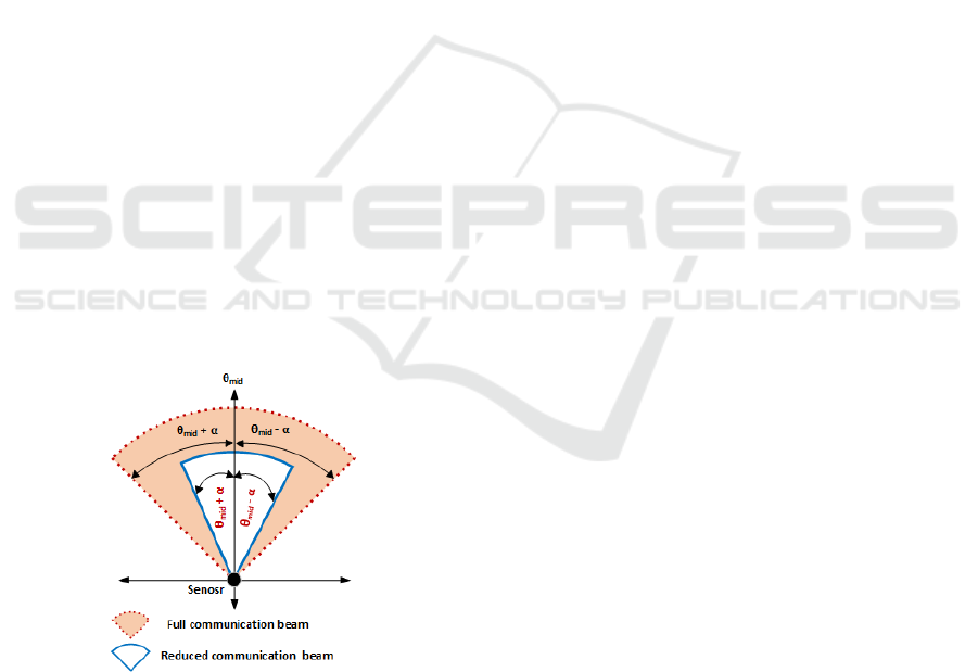
• Θ

mid

is a counterclockwise (CCW) angle between

two rays emanating from x. The ﬁrst ray is a hori-

zontal ray (i.e., parallel to the x-axis) that extends

to the right. The second ray deﬁnes the middle of

x’s transmission beam, see, e.g., Fig. 1.

• For α = α

f ull

, the angle Θ

mid

−α (or, Θ

mid

+α) is

a CCW angle between two rays emanating from x .

The ﬁrst ray is a horizontal ray as above. The sec-

ond ray deﬁnes the start (respectively, the end) of

x’s full range transmission beam (thus, x’s beam

is of width 2α). When α = 180

◦

, the beam is of

width 360

◦

, and node transmission becomes om-

nidirectional. A similar deﬁnition applies when

α = α

red

to describe the reduced transmission

beam.

• R

f ull

(or, R

red

) is the maximum x’s transmission

range when x is in the full (respectively, reduced)

state, and the angle α is sufﬁciently narrow (e.g.,

α = 1

◦

• For a given half-width beam angle α = α

f ull

, the

actual full transmission range of a node x depends

on R

f ull

and the angle α. We use R

f ull

(α) to re-

fer to such an actual transmission range. In gen-

eral, such a transmission range decreases as α in-

creases. Similarly, we use R

red

(α) to refer to a

node’s reduced transmission angle when α = α

red

Figure 1: Node directional communication model.

In Section 7, we experiment with grid networks

having diagonal links. Each grid network has a sink

node located at (x,y)-coordinates (0,0), and the grid

has horizontal (and vertical) links parallel to the x-

axis (respectively, the y-axis), in addition to the di-

agonal links. The horizontal (and vertical) distance

between two horizontally (respectively, vertically) ad-

jacent nodes is set to 100 units. For full energy trans-

mission, we set R

f ull

(α = 1

◦

) = 360 units, and use a

function that reduces the transmission range linearly

so that R

f ull

(α = 180

◦

) = 180 units (for omnidirec-

tional transmission). Likewise, for reduced energy

transmission, we set R

red

(α = 1

◦

) = 180 units, and

red

(α = 180

◦

) = 100 units.

4 PROBLEM FORMULATION

AND CONFIGURATION

APPROACHES

In this section, we start by reviewing (in Section 4.1)

the deﬁnition and key remarks on a WSN path expo-

sure reliability assessment problem, called EXPO-RU

(for path exposure with range uncertainty). The prob-

lem is deﬁned on EH-WSNs where ﬂuctuations in a

node’s stored energy affect primarily its transmission

range.

In the context of designing EH-WSNs with direc-

tional communication nodes, we aim at developing

methods to conﬁgure node transmission dynamically

so as to increase the overall network path exposure

reliability. Achieving this goal is non-trivial since

the EXPO-RU assessment problem has been shown in

(Basabaa and Elmallah, 2021) to be intractable (#P-

hard), and there is no simple optimization criterion

that can be used to adjust the node directionality pa-

rameters so as maximize the overall network reliabil-

ity. As a starting point, and working toward our goal,

we present in Section 4.2 two approaches for adjust-

ing the directionality parameters, so as to obtain good

network reliability performance.

4.1 Review of the EXPO-RU Problem

The EXPO-RU problem is deﬁned in, e.g., (Basabaa

and Elmallah, 2019). Several results on the problem

appears in (Basabaa and Elmallah, 2020).

In the problem, we are given a WSN, and a path

P across the network that we need to monitor against

unauthorized traversal. Nodes that are in close prox-

imity of P can sense the path. Such nodes are called

sensing nodes (speciﬁed as part of the input). The in-

put also speciﬁes an integer k

req

≥ 1 of sensing nodes

that need to sense and report an intrusion event for the

network to succeed in its monitoring task. As men-

tioned above, the EH-WSN reacts to ﬂuctuations in

a node’s stored energy by adjusting the node’s trans-

mission range. The EXPO-RU problem uses a prob-

abilistic graph (G, p) to model the network. In addi-

tion, the problem formulation assumes that different

On Conﬁguring Directional Transmission for Path Exposure Reliability in Energy Harvesting Wireless Sensor Networks

nodes behave independently of each other.

During a short random time interval, the network

G is in some network state S where each node x

is in some state s

∈ { f ull, reduced, f ail}. We use

S = {(x, s

) : x ∈ V, s

∈ { f ull, reduced, f ail}} to refer

to any such network state. Since nodes assume states

independent of each other, the probability that a given

network state S arises is Pr(S) =

∏

(x,s

)∈S

p(x,s

Each network state S is either operating or failed. To

be operating, nodes in S should assign states such that

at least k

req

sensing nodes in S can reach the sink

node. Else, S is in a failed state.

The EXPO-RU problem is called to compute the

probability that the network G is in an operating state

S. We denote such probability by Expo(G, p,P,k

req

or Expo(G, p) for short. Complete enumeration of all

network states can be used to compute Expo(G, p) ex-

actly. However, such an algorithm has a running time

that grows exponentially with the number of nodes in

G. More generally, it has been shown in (Basabaa

and Elmallah, 2021) that the EXPO-RU problem is

#P-hard.

In addition to the concept of network state, we

need the following concepts to discuss our method for

bounding the network reliability measure.

A network conﬁguration C is a partial network state

where some nodes (but not necessarily all) are as-

signed states (an empty conﬁguration is valid) and the

remaining unassigned nodes are free in C. A Pathset

is an operating network conﬁguration that has at least

req

sensing nodes that can reach the sink and monitor

the given intrusion path P. A minpath is a minimal

pathset.

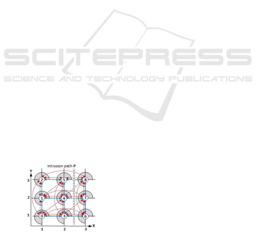
Example. Fig. 2 shows an instance of a 3 × 3 grid

network with one unit of horizontal (or, vertical) spac-

ing. The dashed lines (coloured red) represent com-

munications in full power whereas the solid lines

(coloured blue) represent communications in reduced

power. In Fig. 2, if k

req

= 2, then the conﬁguration

C = {(3,reduced), (4, f ull)} is a pathset and, indeed,

it is a minpath.

Figure 2: An instance of a 3 × 3 grid network.

In this paper, we use the name DirEXPO-RU to

refer to the EXPO-RU problem when nodes employ

directional transmission.

4.2 Approaches for Adjusting

Directional Transmission

Given a node x in a state s ∈ { f ull,reduced}, we

present in this section two approaches for conﬁg-

uring the directionality parameters of the node-state

pair (x,s). We assume that the given problem in-

stance speciﬁes (as part of the input) the angle Θ

mid

that determines the direction of the middle line of x’s

transmission beam (e.g., one may use the direction

of the line segment between x and the sink node).

To adjust the half-width angle α(x,s) for node x in

state s, we experiment with the following two ap-

proaches that aim at maximizing the performance

measure Expo(G, p).

4.2.1 Approach 1

In this approach, we adjust the angle α(x,s) so as to

maximize the out-degree, denoted deg

(x,s), of node

x. Equivalently, we seek to maximize the number of

out-neighbours reachable from node x in state s. We

recall that the actual transmission range R

f ull

(α) (or,

red

(α)) decreases as α increases. The rationale of

this approach is that the more directed links that ex-

ist in any network state S of the resulting probabilis-

tic graph (G, p), the more likely that Expo(G, p) in-

creases.

We next remark that maximizing deg

(x,s) for

the node-state pair (x, s) is a local operation to node

x that does not depend on the directionality setting

of other nodes. Our implementation of this approach

(present in next section) performs sequential search

for ﬁnding an optimized angle α(x,s) in the interval

◦

,180

◦

] in increments of some sufﬁciently small an-

gle δ (e.g., δ = 1

◦

4.2.2 Approach 2

The above approach seeks to maximize the number of

out-neighbours of node x in state s. In this approach,

we consider the quality of such out-neighbours. In

particular, this approach makes an effort to adjust the

angle α(x,s) so as to give preference to include out-

neighbour y of x depending on the quality of the best

found directed path, denoted P

∗

y,sink

, from y to the sink

node. Based on the quality of such a best found path,

we associate with node y a preference weight, de-

noted w(y), that takes on a value that is proportional

to the goodness of the corresponding best found di-

rected path P

∗

y,sink

SENSORNETS 2022 - 11th International Conference on Sensor Networks

We next remark that unlike the ﬁrst approach,

ﬁnding such a best path P

∗

y,sink

depends on the direc-

tionality setting of nodes other than node x (including

node y). To simplify the search for such a best path,

we adopt a heuristic solution that assumes that each

node z, z 6= x, operates in an omnidirectional (full or

reduced) mode.

As done in approach 1, we perform a sequential

search for a good setting of the angle α(x, s) in the

range [1

◦

,180

◦

] in increments of some sufﬁciently

small angle δ (e.g., δ = 1

◦

). At each search step,

the angle α(x,s) is assigned a certain value, and each

node z ∈ V , z 6= x, is assumed to be omnidirectional.

With the angle α(x,s) assigned a speciﬁc value in

each search step, node x can reach a subset of its

possible out-neighbours, denoted S

α(x,s)

. With each

possible out-neighbour y of x assigned a preference

weight w(y), we deﬁne the weight of the set S

α(x,s)

to be w(S

α(x,s)

) =

∑

y∈S

α(x,s)

w(y). Then, the search al-

gorithm selects an angle α(x, s) that gives the highest

w(S

α(x,s)

The details of computing the preference weight

w(y) of a possible out-neighbour y of x follows the

following steps.

1. Let (a, b) be an arc in the probabilistic graph

(G, p) that exists when node a is in state s ∈

{ f ull,reduced}. We recall that typically the

graph G has many parallel arcs since an arc (a, b)

that exists when node a is in the full state may

also exist when a is in the reduced state (and the

two arcs are considered to be different). We asso-

ciate with each such an arc (a,b) a cost, denoted

cost(a,b), that takes on a small value when the

node state probability p(a, s) takes on a high value

(e.g., cost(a,b) = −log p(a, s)).

2. The cost of a directed path P

(y,sink)

from a node y

to the sink, denoted cost(P

(y,sink)

), is the sum of

the costs of its arcs.

3. We set the directed graph G

to be G with node x

deleted. Taking arc costs as distances in G

and

the sink node as a destination, we solve a single-

destination shortest paths problem to ﬁnd a short-

est path from each potential out-neighbour y of x

to the sink. We denote such a shortest path by

∗

y,sink

4. Finally, we assign a preference value w(y) to node

y so that the value is inversely proportional to the

cost(P

∗

y,sink

) (e.g., w(y) = 1/cost(P

∗

y,sink

)).

We conclude this section by noting that the two

above approaches also apply when each node has

multiple states (i.e., not only the basic 3-state model

used to explain the approaches).

5 MORE ALGORITHMIC

DETAILS

In this section, we present a heuristic algorithm,

called HWAS (for half-width angle selection), that

utilizes the two proposed approaches (explained in

Section 4.2) to conﬁgure the transmission beams of

each individual node x in the network given its work-

ing direction Θ

mid

. The devised HWAS algorithm

produces two different types of results based on the

selected approach.

5.1 Algorithm Idea

Consider an instance (G, p) of the DirEXPO-RU

problem with directional parameters DIR

comm

(x) =

{Θ

mid

,α

f ull

,α

red

f ull

red

} for each node x ∈ G,

where Θ

mid

, R

f ull

, and R

red

are given. Our devised

algorithm conﬁgures the directionality parameters for

each individual node x ∈ G by ﬁnding the half-width

angle α(x,s) for node x in state s using Approach 1

and Approach 2.

The algorithm utilizes an associative array, de-

noted Best

, to store such α(x, s) values. In other

words, Best

provides a key-value mapping, where

a key is a tuple (x,s) of node x in state s (e.g.,

s ∈ { f ull,reduced}), and the corresponding value is

α(x,s).

In particular, the algorithm conﬁgures the direc-

tionality parameters of the node-state pair (x , s) by

performing the following steps:

1. Perform a sequential search for a good setting

of the angle α(x,s) in the range [1

◦

,180

◦

] in

increments of some sufﬁciently small angle δ

(e.g., δ = 1

◦

), which implies adjusting the trans-

mission beam of node x in state s to reach a

subset of its possible out-neighbours, denoted

α(x,s)

. After processing all α(x,s), we obtain a set

(x,s)

,...,S

180

(x,s)

} of possible out-neighbours

of x that correspond to values of α(x , s).

2. We evaluate the obtained set, and select a member

α(x,s)

using either Method-1 or Method-2 (ex-

plained below).

3. Then, we set Best

(x,s) = α(x, s) that corresponds

to the best subset S

α(x,s)

of out-neighbours of x in

state s.

5.1.1 Method-1

This method is based on Approach 1 (explained in

Section 4.2). It is a baseline method that selects

α(x,s) for each node x ∈ G based on the number

of out-neighbours of x. The approach aims at

On Conﬁguring Directional Transmission for Path Exposure Reliability in Energy Harvesting Wireless Sensor Networks

increasing the reachablity of node x to maximize

the performance measure Expo(G, p). In particular,

Method-1 works by selecting a member S

α(x,s)

(x,s)

,...,S

180

(x,s)

} that has the highest number

of out-neighbours of x. We set Best

(x,s) = α(x,s)

corresponding to the selected member S

α(x,s)

5.1.2 Method-2

This method is based on Approach 2. It is a cost-

based method that selects a subset S

α(x,s)

for each

node x ∈ G based on good out-neighbours of x in state

s, and hence can improve the performance measure

Expo(G, p). In particular, Method-2 works by select-

ing a member S

α(x,s)

of the set {S

(x,s)

,...,S

180

(x,s)

}

that has the highest weight, w(S

α(x,s)

), as explained

in Section 4.2. Then, we set Best

(x,s) = α(x , s)

corresponding to the selected member S

α(x,s)

of out-

neighbours of x in state s.

After computing α

f ull

and α

red

for each node

x ∈ G, the actual f ull (respectively, reduced) trans-

mission range of a node x is calculated as explained in

Section 4.2. Therefore, f ull (respectively, reduced)

arcs for each node x ∈ G are added based on node’s

directionality parameters DIR

comm

(x).

Function HWAS(G, p)

Input: An instance (G, p) of the DirEXPO-RU

problem, and DIR

comm

(x) for each node x ∈ G

Output: Compute α(x,s) where x ∈ G and

s ∈ { f ull,reduced}

1. set Best

= {}

2. foreach (node x ∈ G)

{

3. foreach (node state s ∈ { f ull, reduced})

{

4. for (α = 1

◦

to 180

◦

step δ)

{

5. ﬁnd set {S

(x,s)

,...,S

180

(x,s)

} of subsets

of out-neighbours of x as explained in

the text

}

6. evaluate the obtained set and select a subset

α(x,s)

for x in state s using Method-1 or

Method-2 as explained in the text

7. set Best

[(x,s)] = α(x,s) that corresponds to

α(x,s)

}

8. return Best

Figure 3: Function HWAS for the DirEXPO-RU problem.

5.2 Algorithm Details

Fig. 3 shows a pseudo code for function HWAS. Step

1 initializes array Best

used to store α(x,s) for all

nodes in G. The nested loop in Steps 2 and 3 iter-

ates over each node-state pair (x,s) to ﬁnd its half-

width angle α(x, s). Steps 4 and 5 perform a sequen-

tial search for a good setting of an angle α(x,s) in

the range [1

◦

,180

◦

] (in increment of δ = 1

◦

). This

process generates a set {S

(x,s)

,...,S

180

(x,s)

} of pos-

sible subsets for node x’s neighbours. Step 6 eval-

uates each generated set, and selects a subset S

α(x,s)

using either Method-1 or Method-2. Step 7 sets

Best

(x,s) = α(x,s) corresponding to the best subset

α(x,s)

of the out-neighbours of x in state s. Finally

Step 9 returns Best

5.3 Running Time

Consider an input problem instance on a 3-state net-

work with n nodes. Denote by d

max

the maximum

possible out-degree of any node (d

max

≤ n−1). Thus,

the maximum possible number of arcs in the network

is m ≤ d

max

(n − 1).

Method-1 iterates a ﬁxed number of times (de-

pending on the increment angle δ) over every node-

state pair (x, s). Each iteration examines at most d

max

possible out-neighbours of x. Thus, the algorithm re-

quires O(n · d

max

) time.

Similarly, Method-2 iterates over every node-state

pair (x, s). Each iteration solves a single-destination

shortest paths in time Θ(n + m) time (see, e.g., (Cor-

men et al., 2009)). Thus, the algorithm requires

O(n · (n + m)) time.

6 COMPUTING BOUNDS

One main contributions in this work is obtain-

ing lower bounds (LBs) on Expo(G, p, k

req

) for the

DirEXPO-RU problem where each input graph G

is constructed by our devised HWAS conﬁguration

methods. To compute the Expo measure for any given

problem instance, we use an iteratively improvable

method, called the factoring method. Reference (Ball

et al., 1995) is among the early references to this gen-

eral method. Subsequently the method has been used

to obtain lower and upper bounds on many reliability

problems, including the class of path exposure prob-

lems (see, e.g., (Elmorsy et al., 2013; Basabaa and El-

mallah, 2019)). In (Elmorsy et al., 2013), the authors

adapt the factoring method to compute lower bounds

(LBs) and upper bounds (UBs) of the EXPO problem

SENSORNETS 2022 - 11th International Conference on Sensor Networks

by generating s-disjoint pathsets and cutsets, respec-

tively.

In more details, the factoring algorithm systemati-

cally generates a set of pairwise statistical disjoint (s-

disjoint, for short) conﬁgurations that can be used to

obtain bounds from the sum of disjoint products. We

call two conﬁgurations C

and C

s-disjoint if at least

one node, say x, that appears in both C

and C

is as-

signed two different states in the two conﬁgurations.

So, Pr(C

) + Pr(C

) is the probability of obtaining at

least C

and/or C

. For the DirEXPO-RU problem,

e.g., the conﬁgurations C

= {(1, reduced),(2, f ail)},

and C

= {(1, f ull),(2, f ail)} are s-disjoint since

node 1 is assigned two different states in C

and C

For the EXPO-RU problem (with omnidirectional

transmission), the work in (Basabaa and Elmallah,

2019) develops an efﬁcient function, called E2P (for

extension to a pathset), that extends (if possible) a

given conﬁguration C to a pathset. The authors use the

function within the factoring method to obtain LBs on

the solutions. In this context, the method generates a

set {P

,··· ,P

} of pathsets such that

Expo(G, p,k

req

) ≥

∑

i=1

Pr(P

) (1)

In the next section, we present results based on us-

ing this latter method to compute LBs on problem in-

stances generated by our HWAS conﬁguration meth-

ods.

7 NUMERICAL RESULTS

In this section, we present selected numerical re-

sults to evaluate and compare the performance of

the devised directional transmission conﬁguration ap-

proaches.

Test networks. The selected results are for a class

of networks that can be viewed as extended 2-

dimensional square grid networks (denoted x-grids).

Any such W×W network G has W rows (and columns)

indexed as 0,1,2,··· ,W − 1 from bottom to top (re-

spectively, left to right). Each node has (x,y)-

coordinates. The sink node is placed at the origin at

coordinates (0,0). Rows (respectively, columns) run

horizontally (respectively, vertically) parallel to the x-

axis (respectively, the y-axis). The horizontal (or ver-

tical) distance between two consecutive nodes in the

grid is set to 100 units.

As explained in Section 3.3, when a node is in

the full energy state its actual transmission range is

assumed (for simplicity) to decrease linearly from

f ull

(α = 1

◦

) = 360 units to R

f ull

(α = 180

◦

) = 180

units (the omnidirectional case) as the half-width

beam angle α increases. Thus, e.g., with omnidi-

rectional transmission of an internal node x, the node

can reach 8 other nodes (corresponding to 4 horizon-

tal and vertical neighbours, and 4 diagonal nodes).

Likewise, when a node is in the reduced energy state

its actual transmission range decreases linearly from

red

(α = 1

◦

) = 180 units to R

red

(α = 180

◦

) = 100

units as the half-width beam angle α increases. Thus,

with omnidirectional transmission of an internal node

x, the node can reach 4 other nodes. In each x-grid,

the intrusion path P runs vertically between the right-

most two columns. Only nodes that lie on the imme-

diate left and right of P sense the path.

Node-state Probabilities. We obtain results with

95% conﬁdence and each point in each obtained curve

is the average of 20 runs, where each run assigns to

each node x random p

f ull

(x) and p

red

(x) such that

f ull

(x) + p

red

(x) + p

f ail

(x) = 1 and each run com-

pletes within 71 seconds.

Reliability Lower Bounding Method. In each run, a

LB on Expo(G, p) is obtained by the factoring algo-

rithm after performing 1000 iterations.

Graph Legend. Labels Method-1 and Method-2 re-

fer to results obtained using our devised HWAS algo-

rithm based on Approach 1 and Approach 2 , respec-

tively. The Omni label refer to results obtained using

omnidirectional transmission.

7.1 Effect of Varying Θ

mid

In this set of experiments, we explore the ability of

our two devised approaches to conﬁgure the beam-

widths of each node so as to achieve good LBs on the

exposure reliability measure. We utilize a 6 × 6 x-

grid, and vary Θ

mid

in the range [0

◦

,360

◦

] (all nodes

use the same Θ

mid

value). We recall that for each

node x and state s ∈ { f ull,reduced}, the proposed

approaches are used to conﬁgure the angles α(x,s),

and consequently the out-neighbours of node x.

Fig. 4a presents a histogram of the average num-

ber of links in the network that results from using ran-

dom node-state probabilities (explained above). The

average number of links achieved by the omnidirec-

tional conﬁguration is constant (independent of Θ

mid

Method-1 has a particular strength in maximizing the

out-degree of each node, Thus, it achieves the high-

est average number of total links in the network.

Method-2, however, produces a comparable number

of links in the graph.

Fig. 4b presents curves of the average LB on the

On Conﬁguring Directional Transmission for Path Exposure Reliability in Energy Harvesting Wireless Sensor Networks

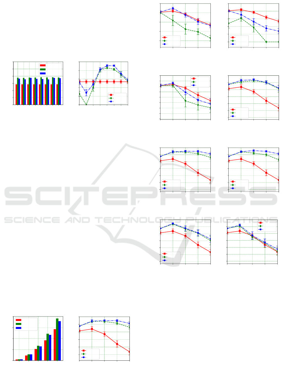
computed Expo(G, p) measure. Method-2 has a par-

ticular strength in selecting for each node x reacha-

bility to out-neighbours that are deemed to be good

in reaching the sink node. Thus, one expects the re-

sulting LBs to outperform LBs obtained from the two

other methods. This expected behaviour is conﬁrmed

in the ﬁgure.

0 45 90 135 180 225 270 315

mid

= 180

150

300

450

600

750

900

Number of links

Omni

Method-1

Method-2

(a) Number of links

0 45 90 135 180 225 270 315

mid

= 180

0.0

0.2

0.4

0.6

0.8

1.0

Exposure (LB)

Omni

Method-1

Method-2

(b) Exposure

Figure 4: Links and exposure versus Θ

mid

∈ [0

◦

,360

◦

7.2 Effect of Varying Network Size

Here, we show the effects of using different networks

of size W × W, where W ∈ [2, 6] and Θ

mid

= 180

◦

on the obtained number of links and exposure. The

proposed approaches are used to conﬁgure the trans-

mission beams of each node for both the f ull and

reduced power states. Fig. 5a and Fig. 5b show the

obtained number of links and exposure, respectively,

for all methods: Method-1, Method-2, and the Omni

method.

Fig. 5a shows that the number of links increases

as network’s size increases for all used methods as

a large network will have a higher number of nodes,

and hence more links. However, Method-1 obtains

the highest number of links compared to Method-2

and the Omni method. Fig. 5b shows that the ob-

tained results by Method-1 and Method-2 outperform

the Omni method for different network sizes. The

results illustrate the advantages of using directional

sensors over omnidirectional as they provide a higher

level of tunability needed in optimizing their perfor-

mance when network’s size increases.

2 3 4 5 6

Network size

150

300

450

600

Number of links

Omni

Method-1

Method-2

(a) Number of links

2 3 4 5 6

Network size

0.5

0.6

0.7

0.8

0.9

1.0

Exposure (LB)

Omni

Method-1

Method-2

(b) Exposure

Figure 5: Links and exposure versus network size.

2 3 4 5 6

Network size

0.2

0.4

0.6

0.8

1.0

Exposure (LB)

Omni

Method-1

Method-2

(a) Θ

mid

= 0

◦

2 3 4 5 6

Network size

0.0

0.2

0.4

0.6

0.8

1.0

Exposure (LB)

Omni

Method-1

Method-2

(b) Θ

mid

= 45

◦

2 3 4 5 6

Network size

0.2

0.3

0.4

0.5

0.6

0.7

0.8

0.9

1.0

Exposure (LB)

Omni

Method-1

Method-2

mid

= 90

◦

2 3 4 5 6

Network size

0.4

0.5

0.6

0.7

0.8

0.9

1.0

Exposure (LB)

Omni

Method-1

Method-2

(d) Θ

mid

= 135

◦

2 3 4 5 6

Network size

0.4

0.5

0.6

0.7

0.8

0.9

1.0

Exposure (LB)

Omni

Method-1

Method-2

(e) Θ

mid

= 180

◦

2 3 4 5 6

Network size

0.4

0.5

0.6

0.7

0.8

0.9

1.0

Exposure (LB)

Omni

Method-1

Method-2

(f) Θ

mid

= 225

◦

2 3 4 5 6

Network size

0.4

0.5

0.6

0.7

0.8

0.9

1.0

Exposure (LB)

Omni

Method-1

Method-2

(g) Θ

mid

= 270

◦

2 3 4 5 6

Network size

0.4

0.5

0.6

0.7

0.8

0.9

1.0

Exposure (LB)

Omni

Method-1

Method-2

(h) Θ

mid

= 315

◦

Figure 6: Obtained bounds versus network size.

7.3 Identifying Good Working Direction

mid

Conﬁguring the direction of the transmission beam

center (determined by the angle Θ

mid

) of nodes in the

network is critical for obtaining good performance.

In cases when this parameter is misconﬁgured for a

node, it is hoped that by adapting the beam width the

node can still deliver acceptable performance.

In this set of experiments, we examine this as-

pect when using W×W x-grids and varying W in the

range [2,6]. Since the sink node is placed at the (x,y)-

SENSORNETS 2022 - 11th International Conference on Sensor Networks

coordinate (0,0), the direction of the line between a

node x and the sink varies in the range [180

◦

,270

◦

]

(180

◦

for nodes on the x-axis, and 270

◦

for nodes on

the y-axis).

Fig. 6 shows detailed obtained results when

changing Θ

mid

in the range [0

◦

,360

◦

]. The results

show that directional settings outperform the omni-

directional setting when all nodes are oriented so that

mid

∈ [180

◦

,270

◦

]. The results also show that even

when Θ

mid

= 90

◦

(a setting that can be viewed as a

misconﬁguration, given the sink position), the work-

ing of Method-1 and Method-2 have been able to ad-

just the angle α of each node and the obtained LBs

are comparable with the omnidirectional case. The

results also point to the importance of adjusting the

beam-width 2α based on the quality of the obtained

routes to the sink (as considered in Approach 2).

0.0 0.1 0.2 0.3 0.4 0.5

Node state probability

0.0

0.2

0.4

0.6

0.8

1.0

Exposure

Omni

Method-1

Method-2

(a) k

req

= 1 and Θ

mid

= 180

◦

0.0 0.1 0.2 0.3 0.4 0.5

Node state probability

0.0

0.2

0.4

0.6

0.8

1.0

Exposure

Omni

Method-1

Method-2

(b) k

req

= 3 and Θ

mid

= 180

◦

Figure 7: Exposure versus node state probability.

7.4 Exposure versus Node State

Probability

Here, we compare directional transmission with

omnidirectional transmission as we set p

f ull

(x) =

red

(x) = p for each node x, and vary p in the range

[0.0,0.5]. The probability p here can be viewed as the

node’s operating (either in the f ull or reduced sates)

probability. We note that low p values correspond to

cases where the fraction of time when nodes in the

network operate in the full or reduced energy states is

small. This can happen, e.g., because nodes can not

harvest enough energy, or nodes decide to conserve

power.

The experiments use a 6 × 6 x-grid with k

req

1 (Fig. 7a), and k

req

= 3 (Fig. 7b). In all cases,

for any value of p, directional transmission achieves

higher average LB on Expo(G, p) than omnidirec-

tional transmission. The results show the advantage

of utilizing and properly conﬁguring directional EH-

WSNs. The curves also show that directional net-

works are capable of having an exposure reliability

that exceeds the operating probability of any single

node in the network.

8 CONCLUSIONS

In this paper, we consider a fundamental problem

on conﬁguring the transmission beams of nodes in a

WSN that employs energy harvesting (EH) to achieve

prolonged operating time. We take the overall net-

work reliability for a path exposure problem as an ob-

jective function that we seek to maximize. The pro-

posed approaches have shown the advantages of using

directional transmission over omnidirectional trans-

mission. For future work, we propose investigating

the design of more comprehensive dynamic conﬁgu-

ration mechanisms of such networks for a variety of

WSN reliability problems.

REFERENCES

Adu-Manu, K., Adam, N., Tapparello, C., Ayatollahi, H.,

and Heinzelman, W. (2018). Energy-harvesting wire-

less sensor networks (EH-WSNs): A review. ACM

Transactions on Sensor Networks, 14:1–50.

Amac Guvensan, M. and Gokhan Yavuz, A. (2011). On

coverage issues in directional sensor networks: A sur-

vey. Ad Hoc Networks, 9(7):1238–1255.

Ball, M. O., Colbourn, C. J., and Provan, J. (1995). Network

reliability. In Ball, M. O., Magnanti, T. L., Monma,

C. L., and Nemhauser, G. L., editors, Handbook of

Operations Research: Network Models, pages 673–

762. Elsevier North-Holland.

Basabaa, A. and Elmallah, E. S. (2019). Bounds on path

exposure in energy harvesting wireless sensor net-

works. In 2019 IEEE Wireless Communications and

Networking Conference (WCNC).

Basabaa, A. and Elmallah, E. S. (2020). Bounding path ex-

posure in energy harvesting wireless sensor networks

using pathsets and cutsets. In The 45th IEEE Confer-

ence on Local Computer Networks (LCN).

Basabaa, A. and Elmallah, E. S. (2021). Upper bounds on

path exposure in EH-WSNs with variable transmis-

sion ranges. In The 46th IEEE Conference on Local

Computer Networks (LCN).

Clouqueur, T., Phipatanasuphorn, V., Ramanathan, P., and

Saluja, K. K. (2003). Sensor deployment strategy for

detection of targets traversing a region. Mobile Net-

works and Applications, 8:453–461.

Cormen, T., Leiserson, C., Rivest, R., and Stein, C. (2009).

Introduction to Algorithms. McGraw Hill, MIT Press,

third edition.

Duan, Z., Tao, L., and Zhang, X. (2019). Energy efﬁcient

data collection and directional wireless power trans-

fer in rechargeable sensor networks. IEEE Access,

7:178466–178475.

Elmorsy, M., Elmallah, E. S., and AboElFotoh, H. M.

(2013). On path exposure in probabilistic wireless

sensor networks. In The 38th IEEE Conference on

Local Computer Networks (LCN).

On Conﬁguring Directional Transmission for Path Exposure Reliability in Energy Harvesting Wireless Sensor Networks

Jakobsen, M. K., Madsen, J., and Hansen, M. R. (2010).

DEHAR: A distributed energy harvesting aware rout-

ing algorithm for ad-hoc multi-hop wireless sensor

networks. In 2010 IEEE International Symposium on

”A World of Wireless, Mobile and Multimedia Net-

works” (WoWMoM), pages 1–9.

Li, W., Gao, H., Liu, Y., Jia, B., and Huang, B. (2020). A

priority task scheduling algorithm based on residual

energy in EH-WSNs. In 2020 16th International Con-

ference on Mobility, Sensing and Networking (MSN),

pages 43–48.

Liu, L., Zhang, X., and Ma, H. (2009). Minimal exposure

path algorithms for directional sensor networks. In

GLOBECOM 2009 - 2009 IEEE Global Telecommu-

nications Conference, pages 1–6.

Mart

ınez, G., Li, S., and Zhou, C. (2014). Wastage-

aware routing in energy-harvesting wireless sensor

networks. IEEE Sensors Journal, 14:2967–2974.

Megerian, S., Koushanfar, F., Qu, G., Veltri, G., and

Potkonjak, M. (2002). Exposure in wireless sensor

networks: theory and practical solutions. Wireless

Network, 8:443–454.

Peng, S. and Low, C. P. (2013). Energy neutral routing for

energy harvesting wireless sensor networks. In 2013

IEEE Wireless Communications and Networking Con-

ference (WCNC), pages 2063–2067.

Peng, S., Wang, T., and Low, C. P. (2015). Energy neu-

tral clustering for energy harvesting wireless sensors

networks. Ad Hoc Networks, 18:1 – 16.

Sudevalayam, S. and Kulkarni, P. (2011). Energy harvesting

sensor nodes: Survey and implications. IEEE Com-

munications Surveys Tutorials, 13(3):443–461.

Tao, D. and Wu, T.-Y. (2015). A survey on barrier coverage

problem in directional sensor networks. IEEE Sensors

Journal, 15(2):876–885.

Zhang, L., Tang, J., and Zhang, W. (2009). Strong barrier

coverage with directional sensors. In GLOBECOM

2009 - 2009 IEEE Global Telecommunications Con-

ference, pages 1–6.

Zhu, X., Li, J., Zhou, M., and Chen, X. (2019). Optimal de-

ployment of energy-harvesting directional sensor net-

works for target coverage. IEEE Systems Journal,

13(1):377–388.

SENSORNETS 2022 - 11th International Conference on Sensor Networks