A Step Towards the Explainability of Microarray Data for Cancer

Diagnosis with Machine Learning Techniques

Adara S. R. Nogueira

, Artur J. Ferreira

1,3 a

and M

ario A. T. Figueiredo

2,3 b

ISEL, Instituto Superior de Engenharia de Lisboa, Instituto Polit

ecnico de Lisboa, Portugal

IST, Instituto Superior T

ecnico, Universidade de Lisboa, Portugal

Instituto de Telecomunicac¸

oes, Lisboa, Portugal

Keywords:

Machine Learning, Feature Selection, Feature Discretization, Microarray Data, Cancer Explainability.

Abstract:

Detecting diseases, such as cancer, from from gene expression data has assumed great importance and is a

very active area of research. Today, many gene expression datasets are publicly available, which consist of

microarray data with information on the activation (or not) of thousands of genes, in sets of patients that have

(or not) a certain disease. These datasets consist of high-dimensional feature vectors (very large numbers of

genes), which raises difﬁculties for human analysis and interpretation with the goal of identifying the most

relevant genes for detecting the presence of a particular disease. In this paper, we propose to take a step towards

the explainability of these disease detection methods, by applying feature discretization and feature selection

techniques. We accurately classify microarray data, while substantially reducing and identifying subsets of

relevant genes. These small subsets of genes are thus easier to interpret by human experts, thus potentially

providing valuable information about which genes are involved in a given disease.

1 INTRODUCTION

The problem of analysing a patient’s DNA data to

identify the presence/absence of speciﬁc genes, in-

dicative of certain diseases, such as cancer, is an

active topic of research where machine learning

tools play an important role. Many gene expres-

sion datasets are publicly available (Alonso-Betanzos

et al., 2019)

, which include microarray data with in-

formation on the activation (or not) of thousands of

genes, in sets of patients who have (or not) a certain

disease. Ideally, one would like to use these datasets

to learn to predict the presence of a given disease on

new patients, given their microarray data, and to iden-

tify the most relevant genes for that purpose. How-

ever, these datasets are very high-dimensional, which

raises difﬁculties for human experts to interpret the

data. It is laborious to identify the most important

genes that explain the presence of a particular disease.

In addition to their high dimensionality, these datasets

have a small number of instances due to the high cost

of acquiring new instances.

Applying classiﬁcation techniques directly on

https://orcid.org/0000-0002-6508-0932

https://orcid.org/0000-0002-0970-7745

http://csse.szu.edu.cn/staff/zhuzx/Datasets.html

these datasets poses challenges due to the “curse of

dimensionality” issues (Bishop, 1995). The perfor-

mance of the classiﬁers is sub-optimal and it is often

not possible to determine, in detail, which genes are

relevant to detect a given disease. In this paper, we

apply feature discretization (FD) (Garcia et al., 2013),

feature selection (FS) (Duda et al., 2001; Guyon et al.,

2006), to microarray datasets, to overcome these is-

sues. Moreover, analysing the resulting feature sub-

sets allows identifying the smallest subset of features

that are indicative of a given disease. These subsets

allow human interpretability of the data. Figure 1

depicts the main steps of the approach taken in this

work.

Figure 1: The key steps of the proposed approach.

The remainder of this paper is organized as fol-

362

Nogueira, A., Ferreira, A. and Figueiredo, M.

A Step Towards the Explainability of Microarray Data for Cancer Diagnosis with Machine Learning Techniques.

DOI: 10.5220/0010980100003122

In Proceedings of the 11th International Conference on Pattern Recognition Applications and Methods (ICPRAM 2022), pages 362-369

ISBN: 978-989-758-549-4; ISSN: 2184-4313

lows. Section 2 overviews the state-of-the-art on

DNA microarray techniques and reviews some ap-

proaches. The proposed approach as well as the mi-

croarray datasets are presented in Section 3. The ex-

perimental evaluation is reported in Section 4. Fi-

nally, Section 5 ends the paper with concluding re-

marks and directions for future work.

2 DNA MICROARRAYS

In this section, we review the key aspects regarding

the DNA Microarray technique and data generation

(Section 2.1) as well as some approaches to deal with

this type of data (Section 2.2).

2.1 The DNA Microarray Technique

Every biological organism has a set of genes encoded

in its DNA. These may be expressed, i.e., active,

in different cells at different points in time. In the

context of biological/medical research, it’s important

to understand which genes are being expressed (ac-

tive/inactive) in a given cell, at a given point in time.

However, living beings have thousands of genes, e.g.,

humans have approximately 21000 (Forero and Pa-

trinos, 2020; Weinberg, 2014). Each one of these

genes is responsible for encoding a protein, which is

in charge of a speciﬁc functionality. Given the com-

plexity and amount of information, it is currently in-

feasible to analyse this data one gene at a time. Even

if it were possible, it would take a very long time and

the efﬁciency and accuracy of the analysis would be

extremely low.

The DNA microarray technique (Simon et al.,

2003) addresses this issue. A DNA microarray allows

researchers and healthcare professionals to carry out

an investigation on thousands of genes at a time, i.e.,

in one single experiment

and determine which genes

are being expressed by a cell. A DNA microarray has

the following characteristics:

• a microarray is a solid surface with thousands of

spots arranged in well-ordered columns and rows;

• each spot on this microarray characterizes only

one gene and contains multiple strands of the

same DNA, i.e. the DNA sequence is unique;

• each spot location and its respective DNA se-

quence is recorded in a database.

DNA microarrays can identify dissimilarities be-

tween cancer cells and healthy cells, more specif-

https://learn.genetics.utah.edu/content/labs/

microarray/

ically, which genes in a cancer cell are being ex-

pressed, but not in a healthy cell.

Figure 2: Overview of the DNA Microarray Technique.

Figure 2 presents an overview of the DNA mi-

croarray technique. First, it’s necessary to extract

the ribonucleic acid (RNA) from the samples cells

and then draw out the messenger RNA (mRNA) from

the existing RNA, because only the mRNA devel-

ops gene expression. Then, a DNA copy is made

from the mRNA with the aid of the reverse transcrip-

tase enzyme, which will generate the complementary

DNA (CDNA). In this process, a label is added in the

CDNA representing each cell sample, e.g., a ﬂuores-

cent red for the cancer cell and a ﬂuorescent green

for the healthy cell. This step is necessary because

DNA is a more stable molecule than RNA and the

labelling allows identifying the genes in each sam-

ple later. Both CDNA types previously created are

added to the DNA microarray and because each spot

of it already has many unique CDNA. When mixed

together they will base pair each other due to the

DNA property, designated complementary base pair-

ing. This process is denominated “hybridization”.

Not all CDNA strands will bind to each other, some

may not hybridize therefore they need to be washed

off. Finally, the DNA microarray is analyzed with a

scanner, which can ﬁnd patterns of hybridization by

detecting the ﬂuorescent colors. As a result, we can

observe the following:

• only a few red CDNA molecules bound to a spot,

which means the gene was being expressed only

in the red (cancer) cell;

• only a few green CDNA molecules bound to an-

other spot, which means the gene was being ex-

pressed only in the green (healthy) cell;

• some of both red and green CDNA molecules

bound to a single spot on the microarray (forming

a yellow spot), which means the gene was being

expressed both in the cancer and the healthy cell;

• several spots of the microarray don’t have a single

red or green CDNA strand bound to it, because

the gene is not being expressed in either cell.

The red color on a spot indicates the higher produc-

tion of mRNA in the cancer cell compared to the

healthy cell. On the other hand, the green color spec-

iﬁes the higher production of mRNA in the healthy

A Step Towards the Explainability of Microarray Data for Cancer Diagnosis with Machine Learning Techniques

363

cell as compared to the cancer cell. However, a yel-

low spot suggests that the gene is expressed equally

in both cells and therefore, they are not relevant as

the cause of the disease, because when the healthy

cell becomes cancerous its activity does not undergo

a change. Using DNA microarray, we can analyze

a large amount of genes at the same time, ﬁnd which

genes are being expressed and decide on a better prog-

nosis based on the previous analyzes.

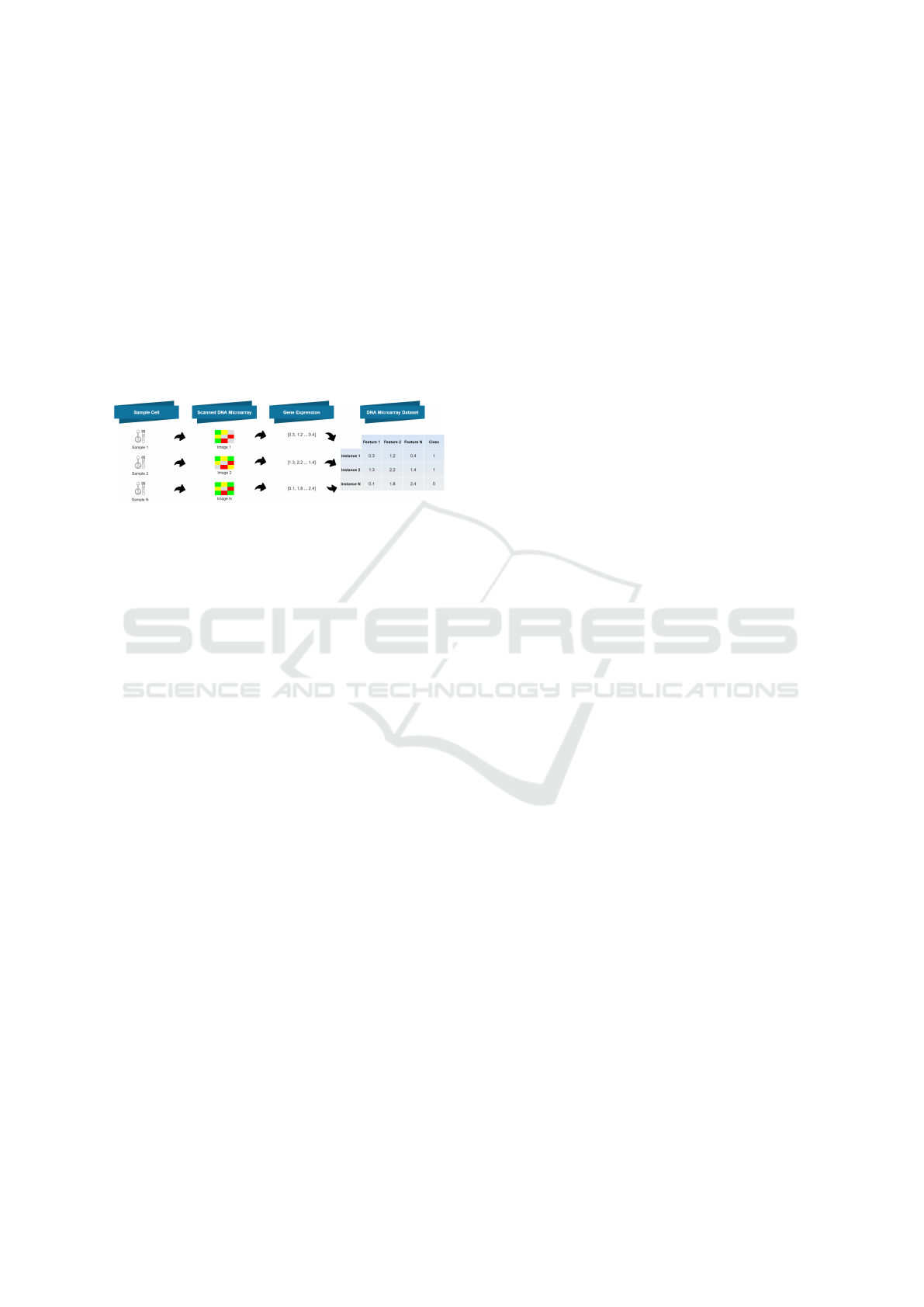
Figure 3 depicts the process of generating a

dataset from the use of the DNA microarray technique

mentioned in Figure 2. The datasets considered in this

work are obtained with this process.

Figure 3: Dataset generation from DNA Microarray.

2.2 Related Approaches

In the last decades, there has been considerable re-

search on microarray data classiﬁcation for cancer

diagnosis (Alonso-Betanzos et al., 2019; Yip et al.,

2011; Statnikov et al., 2005b). Many unsupervised

and supervised FD and FS techniques have been em-

ployed on this type of data, before classiﬁcation takes

place. Since microarray datasets are typically la-

belled, supervised techniques are usually preferred to

unsupervised ones. In this section, we brieﬂy review

some of the existing related work using FD, FS, and

classiﬁcation techniques.

A survey of common classiﬁcation techniques and

related methods to increase their accuracy for mi-

croarray analysis is presented by Alonso-Betanzos

et al. (2019); Yip et al. (2011). The experimental

evaluation is carried out in publicly available datasets.

Saeys et al. (2007) surveyed FS techniques used for

this type of data, showing their adequacy.

It has been found that unsupervised FD performs

well when combined with several classiﬁers. For

instance, the equal frequency binning (EFB) tech-

nique with Na

ıve Bayes (NB) classiﬁer produces very

good results (Witten et al., 2016). It has also been

reported that applying equal interval binning (EIB)

and EFB with microarray data, together with support

vector machines (SVM) classiﬁers, yields good re-

sults (Meyer et al., 2008). The work of Statnikov et al.

(2005a) shows that FS signiﬁcantly improves the clas-

siﬁcation accuracy of multi-class SVM classiﬁers and

other classiﬁcation algorithms.

An FS ﬁlter for microarray data, with an

information-theoretic criterion named double input

symmetrical relevance (DISR), which measures fea-

ture complementarity, was proposed by Meyer et al.

(2008). The reported experimental results on one syn-

thetic dataset and 11 microarray datasets show that the

DISR criterion is competitive with existing FS ﬁlters.

Diaz-Uriarte and Andres (2006) explored FS tech-

niques, such as backwards elimination of features

and classiﬁcation, both using random forests (RF).

The authors applied the chosen method on one simu-

lated and nine real microarray datasets and found that

RF has better performance than other classiﬁcation

methods, such as diagonal linear discriminant analy-

sis (DLDA), K-nearest neighbors (KNN), and SVM.

They also showed that the used FS technique led to a

smaller subset of features than alternative techniques,

namely Nearest Shrunken Centroids and a combined

method of ﬁlter and nearest neighbor classiﬁer.

The work by Li et al. (2018) introduced the use of

large-scale linear support vector machine (LLSVM)

and recursive feature elimination with variable step

size (RFEVSS) as an enhancement to the traditional

FS technique based on SVM with recursive feature

elimination (SVMRFE), which is considered one of

the best methods in the literature, but exhibits large

computational cost. The improved approach consists

in upgrading the RFE by varying the step size with

the goal of reducing the number of iterations (the step

size is kept higher in the initial stages of this process

where non-relevant features are discarded). In addi-

tion, the standard SVM is upgraded to a large-scale

linear SVM and thus accelerating the method of as-

signing weights. The authors compare their approach

to FS with SVM and RF, and use the SVM, NB, KNN

and logistic regression (LR) classiﬁers. These tech-

niques are applied on six microarray datasets and the

approach provides better performance with compara-

ble levels of accuracy, showing that SVM and LR out-

perform the other two classiﬁers.

Recently, in the context of cancer explainability,

Consiglio et al. (2021) considered the problem of

ﬁnding a small subset of features capable of discern-

ing among six classes of instances. These classes may

be healthy or cancerous. The goal was to deﬁne a

comprehensive set of rules based on the most relevant

features (selected by their technique) that can distin-

guish classes based on their gene expressions. The

proposed method combines a genetic algorithm (GA)

to conduct FS and a fuzzy rule-based system to ex-

ecute classiﬁcation on a dataset, with 21 instances,

more than 45 thousand features, and 6 classes. Ten

rules were devised, each one of them taking into ac-

count speciﬁc features, which make them crucial in

ICPRAM 2022 - 11th International Conference on Pattern Recognition Applications and Methods

364

explaining the classiﬁcation results of ovarian cancer

detection.

3 PROPOSED APPROACH

In this section, we present our proposed approach to

handle DNA microarray datasets with machine learn-

ing techniques. Section 3.1 describes the public do-

main datasets used in the experimental evaluation.

Section 3.2 presents the pipeline of techniques that we

apply on the data and the procedures that we follow.

3.1 Microarray Datasets

Table 1 presents the main characteristics of the 11 mi-

croarray datasets used in this work. In this table, n

denotes the number of instances, d indicates the num-

ber of features, and c the number of classes. We also

show the

ratio.

These datasets exhibit the common characteristic

of having many more features than instances, thus

n >> d, making the

ratio quite high for some

datasets, which conveys a challenge in applying ma-

chine learning techniques in these data (Bishop, 1995;

Duda et al., 2001). All datasets have a large number

of features, with d ranging from 2000 to 24481. In ad-

dition, as evidenced by the n column, all datasets have

a small number of instances, with n ranging from 60

to 253.

Table 2 describes the classiﬁcation task for each

of datasets presented in Table 1. We have binary

classiﬁcation and multi-class classiﬁcation problems.

A binary dataset indicates the presence/absence of a

speciﬁc tumor/cancer (such as in the CNS, Colon,

and Ovarian datasets), the re-incidence of a dis-

ease (such as in the Breast dataset), or the diag-

nosis between two types of cancer (such as in the

Leukemia dataset). A multi-class dataset distin-

guishes between different types of cells (such as

in the Leukemia 3c, Leukemia 4c and Lymphoma

datasets), and tumors/cancer (such as in the Lung,

Table 1: Microarray Datasets Characteristics.

Name n d c d/n

Breast 97 24481 2 252.38

CNS 60 7129 2 118.81

Colon 62 2000 2 32.25

Leukemia 72 7129 2 99.01

Leukemia

3c 72 7129 3 99.01

Leukemia 4c 72 7129 4 99.01

Lung 203 12600 5 62.06

Lymphoma 66 4026 3 61.00

MLL 72 12582 3 174.75

Ovarian 253 15154 2 59.89

SRBCT 83 2308 4 27.80

Table 2: Microarray Datasets Clinical Tasks.

Name Description

Breast Breast cancer diagnosis

CNS Central Nervous System tumor diagnosis

Colon Colon tumor diagnosis

Leukemia Acute Lymphocytic Leukemia and

Acute Myelogenous Leukemia diagnosis

Leukemia 3c Distinguishes types of blood cells which became cancerous

Leukemia 4c Distinguishes types of blood cells which became cancerous

Lung Lung cancer diagnosis

Lymphoma Distinguishes subtypes of non-Hodgkin lymphoma

MLL Distinguishes types of acute leukemia, including

Mixed Lineage Leukemia

Ovarian Ovarian cancer diagnosis

SRBCT Distinguishes types of of Small Round Blue Cell Tumors

MLL, and SRBCT datasets).

3.2 Machine Learning Pipeline

The connection between our proposal and the related

work is that we consider the microarray datasets re-

ferred in these studies as well as the most often used

classiﬁers. We also address different data represen-

tation techniques, combining FD and FS techniques,

before classiﬁcation. Our aim is not solely the correct

classiﬁcation (regarding the error rate, false negative

rate, and false positive rate), but also to ﬁnd the sub-

sets of features that are more decisive for the classiﬁ-

cation task. In detail, the steps of our approach are:

• choose which techniques to evaluate, based on the

existing literature;

• build a machine learning pipeline using data rep-

resentation/discretization, dimensionality reduc-

tion and data classiﬁcation techniques;

• compare the performance of each technique;

• and ﬁnally, identify the best suited technique as

well as the best subset of features to the problem

and datasets under consideration.

Figure 4 depicts the machine learning pipeline of

the actions that we apply on the datasets.

Figure 4: The pipeline of the proposed approach.

4 EXPERIMENTAL EVALUATION

This section reports the experimental evaluation of the

proposed approach on the 11 microarray datasets de-

scribed in Table 1 and Table 2. The machine learning

pipeline is depicted in Figure 4. The experimental re-

sults are organized as follows:

A Step Towards the Explainability of Microarray Data for Cancer Diagnosis with Machine Learning Techniques

365

• Section 4.1 describes the baseline classiﬁcation

results without FD and FS techniques, using the

SVM and decision tree (DT) classiﬁers (phases

(a), (d), and (e) of the pipeline). We chose

these classiﬁers since they take rather different ap-

proaches for classiﬁcation.

• Section 4.2 addresses the use of FD techniques

(phases (a), (b), (d), and (e) from the pipeline)

and also reports the experimental results of FS

techniques (phases (a), (c), (d), and (e) of the

pipeline). Finally, it identiﬁes the best parameter

conﬁguration found for each dataset.

• Section 4.3 presents experimental results toward

the explainability of the classiﬁcation, by identify-

ing the best subsets of features for some datasets.

4.1 Baseline Classiﬁcation Results

First, we evaluate the data classiﬁcation phase of the

pipeline, on each dataset. We check the performance

of the selected classiﬁers (SVM and DT) to establish

the baseline results. We have chosen the SVM clas-

siﬁer because it is the classiﬁcation technique that in

the literature reports the best results. We have also

chosen DT because it is a different classiﬁcation ap-

proach, which is seldom applied to this type of data.

As the methodology for training and testing the classi-

ﬁers, we consider the leave-one-out cross-validation

(LOOCV) technique for all the evaluations in this pa-

per. Since the number of instances n is small, we

achieve a better estimate of the generalization error

and the other evaluation metrics, since there is no

standard deviation due to the data sampling procedure

as it happens on standard 10-fold cross-validation.

Table 3 presents the baseline results (no FD nor

FS) with phase (b) of the pipeline being the normal-

ization of all feature values to the range 0 to 1. Ta-

ble 4 shows a similar evaluation for the DT classiﬁer.

In our experiments, we have found that using entropy

as a criterion to build the tree is better than using the

Gini index; we have also found that the initial ran-

dom state parameter set to 42 is the best choice.

These experimental results from Table 3 and Ta-

ble 4 show that DT does not achieve better results

than the SVM classiﬁer (DT only performs better than

SVM on the CNS dataset). Thus, from these experi-

ments and from the existing literature, SVM with lin-

ear kernel seems to be an adequate classiﬁer for this

type of data. It is also preferable to normalize the data

before doing any machine learning tasks.

4.2 Feature Discretization Assessment

In the literature of microarray data and for other types

of data and machine learning problems, the unsuper-

vised EFB method is know to produce adequate re-

sults. Thus, we have carried out some experiments

using this discretization method. Table 5 reports the

results of the SVM classiﬁer on data discretized by

EFB, with different number of bins.

Analyzing these results for all datasets, we con-

clude that EFB discretization yields a small improve-

ment for the SVM classiﬁer (lower standard deviation

in all datasets). Table 6 shows a summary of the re-

sults of the best conﬁgurations of EFB discretization

and SVM/DT classiﬁers. For each dataset, we select

the best conﬁguration found in our experiments.

We now address the use of FS on the normal-

ized features (without discretization). For our experi-

ments, we consider the Laplacian score (LS), Spec-

tral, Fisher Ratio (FiR), and relevance-redundancy

feature selection (RRFS) (Ferreira and Figueiredo,

2012). Table 7 shows the experimental results for the

SVM classiﬁer. RRFS works in unsupervised mode

using the mean-median (MM) relevance metric and

in supervised mode using FiR as metric.

The RRFS method attains the best classiﬁcation

error results. We also achieve considerable dimen-

sionality reduction. For instance, on the Ovarian

dataset, we get a reduction to 4% of the original di-

mensionality: the number of selected features is about

606, from the original set of 15154 features. A similar

result is obtained for the Lymphoma dataset, in which

we keep 2% of the original features.

We now address the joint effect of all the pipeline

phases depicted in Figure 4. Table 8 presents the best

conﬁgurations for each phase and each dataset.

4.3 Explainability of the Data

In this section, we aim to identify the most rele-

vant features for a given dataset, now that we have

acceptable classiﬁcation results on the previous sec-

tions. Figure 5 (top) shows the feature indices that

are chosen more often on the LOOCV procedure for

the Lymphoma and Ovarian datasets. For a dataset

with n instances, each feature can be chosen up to n

times. The importance of a feature to (accurately clas-

sify) a dataset and to explain the classiﬁcation results

is proportional to the number of times that feature is

chosen in this procedure. We show the top 100 fea-

tures. In the bottom of this ﬁgure, we show a similar

plot for the Leukemia and Leukemia 3c datasets. We

now consider all the features in the dataset, displaying

the number of times each feature is chosen. For both

ICPRAM 2022 - 11th International Conference on Pattern Recognition Applications and Methods

366

Table 3: Test error rate (Err) of LOOCV for the SVM classiﬁer. For ﬁve datasets that have a class label of “no cancer”, we

also consider the false negative rate (FNR) and false positive rate (FPR). For the other six datasets, we dont report the FNR

and FPR metrics, because the task is to distinguish between cancer types. The best result is in boldface.

Linear kernel Poly kernel RBF kernel Sigmoid kernel

Dataset Err FNR FPR Err FNR FPR Err FNR FPR Err FNR FPR

Breast 0.31 0.30 0.31 0.33 0.28 0.37 0.37 0.46 0.29 0.47 1.00 0.00

CNS 0.33 0.62 0.18 0.37 0.62 0.23 0.35 1.00 0.00 0.35 1.00 0.00

Colon 0.18 0.27 0.12 0.27 0.55 0.12 0.21 0.50 0.05 0.39 0.82 0.15

Leukemia 0.01 – – 0.03 – – 0.15 – – 0.35 – –

Leukemia 3c 0.04 – – 0.06 – – 0.26 – – 0.47 – –

Leukemia 4c 0.07 – – 0.10 – – 0.32 – – 0.47 – –

Lung 0.05 0.01 0.12 0.05 0.01 0.18 0.09 0.01 0.24 0.32 0.00 1.00

Lymphoma 0.00 – – 0.00 – – 0.00 – – 0.30 – –

MLL 0.03 – – 0.06 – – 0.10 – – 0.61 – –

Ovarian 0.00 0.00 0.00 0.004 0.00 0.01 0.02 0.01 0.02 0.36 0.00 1.00

SRBCT 0.00 – – 0.01 – – 0.07 – – 0.65 – –

Average, X 0.09 0.24 0.15 0.12 0.29 0.18 0.18 0.40 0.12 0.43 0.56 0.43

Std. dev.,σ 0.12 0.23 0.10 0.13 0.26 0.12 0.13 0.37 0.12 0.11 0.47 0.47

Table 4: Test error rate (Err), FNR, and FPR of LOOCV for the DT classiﬁer using entropy as criterion and random state set

to 42, with normalized features in the range 0 to 1. Different values for the max depth parameter are evaluated (the learned

tree maximum allowed depth).

Max Depth=2 Max Depth=5 Max Depth=7 Max Depth=10

Dataset Err FNR FPR Err FNR FPR Err FNR FPR Err FNR FPR

Breast 0.40 0.35 0.45 0.33 0.30 0.35 0.33 0.30 0.35 0.33 0.30 0.35

CNS 0.18 0.48 0.03 0.25 0.33 0.21 0.25 0.33 0.21 0.25 0.33 0.21

Colon 0.18 0.36 0.08 0.19 0.23 0.18 0.19 0.23 0.18 0.19 0.23 0.18

Leukemia 0.26 – – 0.26 – – 0.26 – – 0.26 – –

Leukemia 3c 0.15 – – 0.17 – – 0.17 – – 0.17 – –

Leukemia 4c 0.11 – – 0.15 – – 0.15 – – 0.15 – –

Lung 0.13 0.01 0.06 0.07 0.01 0.12 0.07 0.01 0.12 0.07 0.01 0.12

Lymphoma 0.00 – – 0.00 – – 0.00 – – 0.00 – –

MLL 0.08 – – 0.08 – – 0.08 – – 0.08 – –

Ovarian 0.03 0.01 0.07 0.03 0.01 0.07 0.03 0.01 0.07 0.03 0.01 0.07

SRBCT 0.27 – – 0.17 – – 0.17 – – 0.17 – –

Average, X 0.16 0.24 0.14 0.15 0.18 0.19 0.15 0.18 0.19 0.15 0.18 0.19

Std. dev., σ 0.11 0.19 0.16 0.10 0.14 0.10 0.10 0.14 0.10 0.10 0.14 0.10

Table 5: Test error rate (Err), FNR, and FPR of LOOCV for the SVM classiﬁer (C=1 and kernel=linear) with EFB discretiza-

tion. Different values for the n bins parameter were evaluated (the number of discretization bins).

Num. Bins=2 Num. Bins=3 Num. Bins=4 Num. Bins=5 Num. Bins=6 Num. Bins=7

Dataset Err FNR FPR Err FNR FPR Err FNR FPR Err FNR FPR Err FNR FPR Err FNR FPR

Breast 0.32 0.30 0.33 0.33 0.33 0.33 0.32 0.33 0.31 0.32 0.33 0.31 0.30 0.30 0.29 0.31 0.33 0.29

CNS 0.35 0.71 0.15 0.30 0.62 0.13 0.38 0.71 0.21 0.32 0.62 0.15 0.32 0.62 0.15 0.37 0.67 0.21

Colon 0.18 0.27 0.12 0.18 0.27 0.12 0.16 0.27 0.10 0.15 0.23 0.10 0.15 0.23 0.10 0.16 0.27 0.10

Leukemia 0.01 – – 0.01 – – 0.01 – – 0.01 – – 0.01 – – 0.01 – –

Leukemia 3c 0.03 – – 0.03 – – 0.03 – – 0.03 – – 0.04 – – 0.04 – –

Leukemia 4c 0.08 – – 0.07 – – 0.07 – – 0.07 – – 0.07 – – 0.07 – –

Lung 0.05 0.01 0.18 0.05 0.01 0.18 0.05 0.01 0.18 0.04 0.01 0.18 0.04 0.01 0.18 0.04 0.01 0.18

Lymphoma 0.00 – – 0.00 – – 0.00 – – 0.00 – – 0.00 – – 0.00 – –

MLL 0.04 – – 0.03 – – 0.03 – – 0.03 – – 0.03 – – 0.03 – –

Ovarian 0.004 0.00 0.01

0.00 0.00 0.00 0.00 0.00 0.00 0.00 0.00 0.00 0.00 0.00 0.00 0.00 0.00 0.00

SRBCT 0.00 – – 0.00 – – 0.00 – – 0.00 – – 0.00 – – 0.00 – –

Average, X 0.10 0.26 0.16 0.09 0.25 0.15 0.10 0.26 0.16 0.09 0.24 0.15 0.09 0.23 0.14 0.09 0.26 0.16

Std. dev., σ 0.12 0.26 0.10 0.12 0.23 0.11 0.13 0.26 0.10 0.12 0.23 0.10 0.11 0.23 0.10 0.12 0.25 0.10

datasets, we can observe that only one single feature is

chosen n times (on the LOOCV folds), thus it is iden-

tiﬁed as the most relevant feature (gene) for cancer

detection, to be checked by the clinical staff. After-

ward, we observe a decreasing function that shows the

relative importance of the features to perform classiﬁ-

cation. We observe that only a few features are chosen

n times, being the most relevant in clinical terms.

5 CONCLUSIONS

Cancer detection and classiﬁcation from high-

dimensional DNA microarray data is an important

problem, with many techniques having been success-

fully applied to these problems. However, more than

just classifying the data, it is also important to iden-

tify the most relevant genes for the classiﬁcation task,

A Step Towards the Explainability of Microarray Data for Cancer Diagnosis with Machine Learning Techniques

367

Table 6: Summary of the best results and respective conﬁgurations, for each dataset with normalized features, obtained during

the data representation phase with the EFB discretizer. The * symbol denotes an improvement over the baseline classiﬁcation

results of Table 3 and Table 4, without discretization.

Conﬁgurations

Dataset Classiﬁer Num. Bins Err FNR FPR

Breast SVM 6 0.30* 0.30 0.29

CNS DT 5 0.18 0.33 0.10

Colon SVM 5, 6 0.15* 0.23 0.10

Leukemia SVM, DT 2, 3, 4, 5, 6, 7 0.01 – –

Leukemia 3c SVM 2, 3, 4, 5 0.03* – –

Leukemia 4c SVM 3, 4, 5, 6, 7 0.07* – –

Lung SVM 5, 6, 7 0.04* 0.01 0.18

Lymphoma SVM 2, 3, 4, 5, 6, 7 0.00 – –

MLL SVM 3, 4, 5, 6, 7 0.03 – –

Ovarian SVM 3, 4, 5, 6, 7 0.00 0.00 0.00

SRBCT SVM 2, 3, 4, 5, 6, 7 0.00 – –

Average, X – – 0.07 0.17 0.13

Std. dev., σ – – 0.09 0.14 0.10

Table 7: Test error rate (Err), FNR, and FPR of LOOCV for the SVM classiﬁer (C=1 and kernel=linear) with LS, SPEC, FiR,

and RRFS (with MM and FiR relevance and maximum similarity m

=0.7), with normalized features.

Unsupervised Supervised

LS SPEC RRFS (MM) FiR RRFS (FiR)

Dataset Err FNR FPR Err FNR FPR Err FNR FPR Err FNR FPR Err FNR FPR

Breast 0.33 0.35 0.31 0.32 0.30 0.33 0.31 0.28 0.33 0.31 0.28 0.33 0.31 0.28 0.33

CNS 0.35 0.52 0.26 0.33 0.62 0.18 0.27 0.48 0.15 0.30 0.57 0.15 0.33 0.67 0.15

Colon 0.16 0.27 0.10 0.19 0.32 0.12 0.21 0.36 0.12 0.19 0.32 0.12 0.18 0.27 0.12

Leukemia 0.01 – – 0.01 – – 0.01 – – 0.01 – – 0.01 – –

Leukemia 3c 0.04 – – 0.06 – – 0.04 – – 0.04 – – 0.03 – –

Leukemia 4c 0.08 – – 0.10 – – 0.07 – – 0.07 – – 0.07 – –

Lung 0.05 0.01 0.12 0.05 0.01 0.12 0.05 0.01 0.12 0.04 0.01 0.12 0.05 0.01 0.18

Lymphoma 0.00 – – 0.00 – – 0.03 – – 0.00 – – 0.02 – –

MLL 0.04 – – 0.06 – – 0.03 – – 0.03 – – 0.04 – –

Ovarian 0.00 0.00 0.00 0.00 0.00 0.00 0.004 0.00 0.01 0.00 0.00 0.00 0.00 0.00 0.00

SRBCT 0.02 – – 0.00 – – 0.00 – – 0.00 – – 0.00 – –

Average, X 0.10 0.23 0.16 0.10 0.25 0.15 0.09 0.23 0.15 0.09 0.24 0.14 0.09 0.25 0.16

Std. dev., σ 0.12 0.20 0.11 0.12 0.23 0.11 0.11 0.19 0.10 0.11 0.21 0.11 0.12 0.24 0.11

Table 8: Pipeline’s best conﬁguration found for each dataset.

Pipeline Conﬁguration

Dataset Discretization Selection Classiﬁcation

Breast EFB (n bins=6) RRFS (with FiR; ms=0.7) SVM (C=1; kernel=linear)

CNS EFB (n bins=5) SPEC DT (criterion=entropy, max depth=6, and random state=42)

Colon MDLP LS DT (criterion=entropy, max depth=None, and random state=5)

Leukemia EFB (n bins=2) LS SVM (C=1; kernel=linear)

Leukemia 3c EFB (n bins=2) RRFS (with FiR; ms=0.7) SVM (C=1; kernel=linear)

Leukemia 4c EFB (n bins=3) RRFS (with FiR; ms=0.7) SVM (C=1; kernel=linear)

Lung EFB (n bins=5) FiR SVM (C=1; kernel=linear)

Lymphoma EFB (n bins=2) LS SVM (C=1; kernel=linear)

MLL EFB (n bins=3) RRFS (with MM; ms=0.7) SVM (C=1; kernel=linear)

Ovarian EFB (n bins=3) RRFS (with FiR; ms=0.7) SVM (C=1; kernel=linear)

SRBCT EFB (n bins=2) SPEC SVM (C=1; kernel=linear)

allowing for the human interpretability of the classiﬁ-

cation results. In this work, we have proposed an ap-

proach using feature selection and feature discretiza-

tion techniques, able to identify small subsets of rele-

vant genes for the subsequent classiﬁer. The proposed

approach is based on standard machine learning pro-

cedures, achieves large degrees of dimensionality re-

duction on several public-domain datasets. By using

the LOOCV procedure, identify the features (genes)

that are often more relevant for the classiﬁer decision.

In future work, we will explore supervised fea-

ture discretization techniques. We will also ﬁne tune

the maximum similarity parameter of the RRFS algo-

rithm to further reduce the size of the subsets, allow-

ing medical experts to focus on fewer features.

REFERENCES

Alonso-Betanzos, A., Bol

on-Canedo, V., Mor

an-

Fern

andez, L., and S

anchez-Marono, N. (2019). A

review of microarray datasets: Where to ﬁnd them and

speciﬁc characteristics. Methods in Molecular Biology,

1986(1):65–85.

Bishop, C. (1995). Neural Networks for Pattern Recogni-

tion. Oxford University Press.

ICPRAM 2022 - 11th International Conference on Pattern Recognition Applications and Methods

368

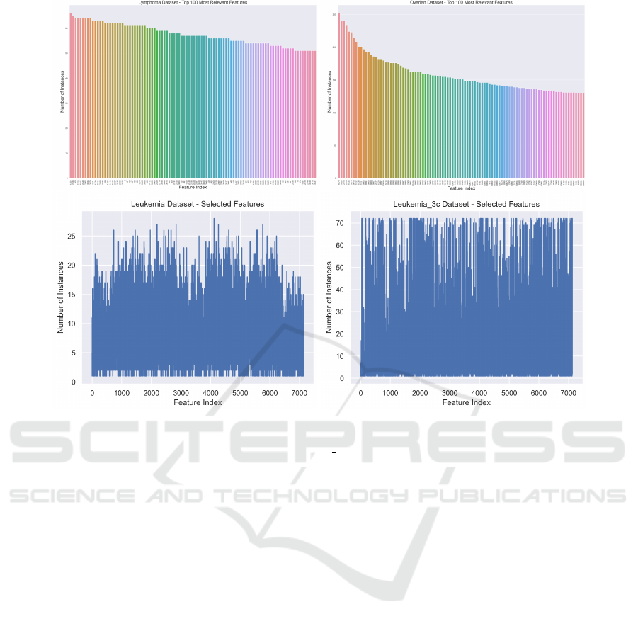
Figure 5: Top: The top-100 of the number of times each feature is chosen/selected on the FS step on the LOOCV procedure

for the Lymphoma (n=66, d=4026) and Ovarian datasets (n=253, d=15154). Bottom: The number of times each feature is

chosen/selected for the Leukemia (n=72, d=7129) and Leukemia 3c datasets (n=72, d=7129).

Consiglio, A., Casalino, G., Castellano, G., Grillo, G., Per-

lino, E., Vessio, G., and Licciulli, F. (2021). Explaining

ovarian cancer gene expression proﬁles with fuzzy rules

and genetic algorithms. Electronics, 10(4):375.

Diaz-Uriarte, R. and Andres, S. (2006). Gene selection

and classiﬁcation of microarray data using random for-

est. BMC bioinformatics, 7(1):1–13.

Duda, R., Hart, P., and Stork, D. (2001). Pattern classiﬁca-

tion. John Wiley & Sons, second edition.

Ferreira, A. and Figueiredo, M. (2012). Efﬁcient feature se-

lection ﬁlters for high-dimensional data. Pattern Recog-

nition Letters, 33(13):1794 – 1804.

Forero, D. and Patrinos, G. (2020). Genome Plasticity

in Health and Disease. Translational and Applied Ge-

nomics. Elsevier Science.

Garcia, S., Luengo, J., Saez, J., Lopez, V., and Herrera, F.

(2013). A survey of discretization techniques: taxon-

omy and empirical analysis in supervised learning. IEEE

Trans. Knowledge and Data Eng., 25(4):734–750.

Guyon, I., Gunn, S., Nikravesh, M., and Zadeh, L.

(2006). Feature extraction, foundations and applica-

tions. Springer.

Li, Z., Xie, W., and Liu, T. (2018). Efﬁcient feature se-

lection and classiﬁcation for microarray data. PloS One,

13(8):e0202167.

Meyer, P., Schretter, C., and Bontempi, G. (2008).

Information-theoretic feature selection in microarray

data using variable complementarity. IEEE Journal of

Selected Topics in Signal Processing, 2(3):261–274.

Saeys, Y., Inza, I., and naga, P. L. (2007). A review of

feature selection techniques in bioinformatics. Bioinfor-

matics, 23(19):2507–2517.

Simon, R., Korn, E., McShane, L., Radmacher, M., Wright,

G., and Zhao, Y. (2003). Design and analysis of DNA

microarray investigations. Springer.

Statnikov, A., Aliferis, C., Tsamardinos, I., Hardin, D., and

Levy, S. (2005a). A comprehensive evaluation of multi-

category classiﬁcation methods for microarray gene ex-

pression cancer diagnosis. Bioinformatics, 21(5):631–

643.

Statnikov, A., Tsamardinos, I., Dosbayev, Y., and Aliferis,

C. (2005b). GEMS: a system for automated cancer di-

agnosis and biomarker discovery from microarray gene

expression data. International Journal of Medical Infor-

matics, 74(7-8):491–503.

Weinberg, R. (2014). The Biology of Cancer. Garland Sci-

ence, second edition.

Witten, I., Frank, E., Hall, M., and Pal, C. (2016). Data min-

ing: practical machine learning tools and techniques.

Morgan Kauffmann, fourth edition.

Yip, W.-K., Amin, S. B., and Li, C. (2011). A Survey of

Classiﬁcation Techniques for Microarray Data Analysis,

pages 193–223. Springer Berlin Heidelberg.

A Step Towards the Explainability of Microarray Data for Cancer Diagnosis with Machine Learning Techniques

369