Comparison of Online Exploration and Coverage Algorithms in

Continuous Space

Malte Z. Andreasen

, Philip I. Holler

, Magnus K. Jensen

and Michele Albano

Department of Computer Science, Aalborg University, Selma Lagerløfs Vej 300, 9220 Aalborg, Denmark

Keywords:

Distributed Exploration, Online Terrain Coverage, Swarm Robotics, Multi Agent Exploration Simulator.

Abstract:

We propose a framework to compare algorithms for multi agent exploration in an unknown continuous 2d

environment. To analyze trade offs we compare algorithms with varying robot hardware requirements. We

showcase our approach on Random Ballistic Walk (RBW), frontier-based exploration (The Next Frontier,

TNF), Spiraling and Selective Backtracking (SSB), and Local Voronoi Decomposition (LVD). Algorithms

that operate in a discrete grid-based space, such as LVD and SSB, are mapped to a continuous space for

comparison with other algorithms. To our knowledge, no other extensive comparison of these exploration

algorithms operating under the same testing environment has been conducted. The algorithms are tested

in a custom 2D physics-driven simulation (Multi Agent Exploration Simulator, MAES), with two types of

maps, namely the Cave map (C-Map) and the Building map (B-Map). The performance of each algorithm is

evaluated in terms of coverage and exploration of the map. Results show that SSB performed the best in terms

of coverage in all tested scenarios. TNF performed the best in terms of exploration, especially on bigger maps.

RBW achieved good results in terms of both coverage and exploration in C-Maps, but not in B-Maps. LVD

performed similarly to RBW in C-Maps, but better in the B-Maps.

1 INTRODUCTION

Collective terrain exploration and coverage using

swarm robotics has many applications such as search

& rescue and surveillance, and in fact it keeps a

prominent role among the use cases for multi agent

algorithms (Schranz et al., 2020; Brambilla et al.,

2013).

The problem of terrain coverage by multiple

agents comprises Ofﬂine Terrain Coverage and On-

line Terrain Coverage (OTC), where online refers to

the terrain being unknown beforehand and thus ex-

plored while the algorithm is executed (Agmon et al.,

2008). In this paper we focus on OTC, and we argue

that many great algorithms have been proposed for

terrain coverage using swarm robotics, however they

are hardly comparable since they model their agents

in very different manners; moreover, we raise the is-

sue of the limited realism introduced by the require-

ments of some of the algorithms in terms of robot

capabilities, such as (i) the environment being con-

https://orcid.org/0000-0002-2338-265X

https://orcid.org/0000-0001-7587-531X

https://orcid.org/0000-0001-9594-0297

https://orcid.org/0000-0002-3777-9981

sidered a grid-like structure that can be maneuvered

by moving from cell to cell (Cheraghi et al., 2020;

Albani et al., 2019) where (ii) the robots cannot suf-

fer from colliding with each other; (iii) communica-

tion between robots has unlimited range and is not

blocked by walls (Kambayashi et al., 2009; Oikawa

et al., 2015); (iv) robots know each other’s location,

not impeded by walls (Kegeleirs et al., 2021), and are

provided with real-time distributed Simultaneous Lo-

calization And Mapping (SLAM) (Gonzalez and Ger-

lein, 2009a).

We propose a framework, and its accompanying

tool Multi Agent Exploration Simulator (MAES), for

taking algorithm simulations one step closer to the

real world by representing their movement space as

a continuous 2D plane, rather than a grid of cells (see

Figure 1), and for mapping the different approaches

on a common ground in terms of hardware capabili-

ties of the robots.

To showcase the approach, we ﬁrst of all (Section

2) provide information regarding selected algorithms,

namely Spiraling and Selective Backtracking (SSB)

from (Gautam et al., 2018), Local Voronoi Decom-

position for Multi-Agent Task allocation (LVD) from

(Fu et al., 2009), The Next Frontier (TNF) from (Co-

Andreasen, M., Holler, P., Jensen, M. and Albano, M.

Comparison of Online Exploration and Coverage Algorithms in Continuous Space.

DOI: 10.5220/0010975900003116

In Proceedings of the 14th International Conference on Agents and Artiﬁcial Intelligence (ICAART 2022) - Volume 1, pages 527-537

ISBN: 978-989-758-547-0; ISSN: 2184-433X

527

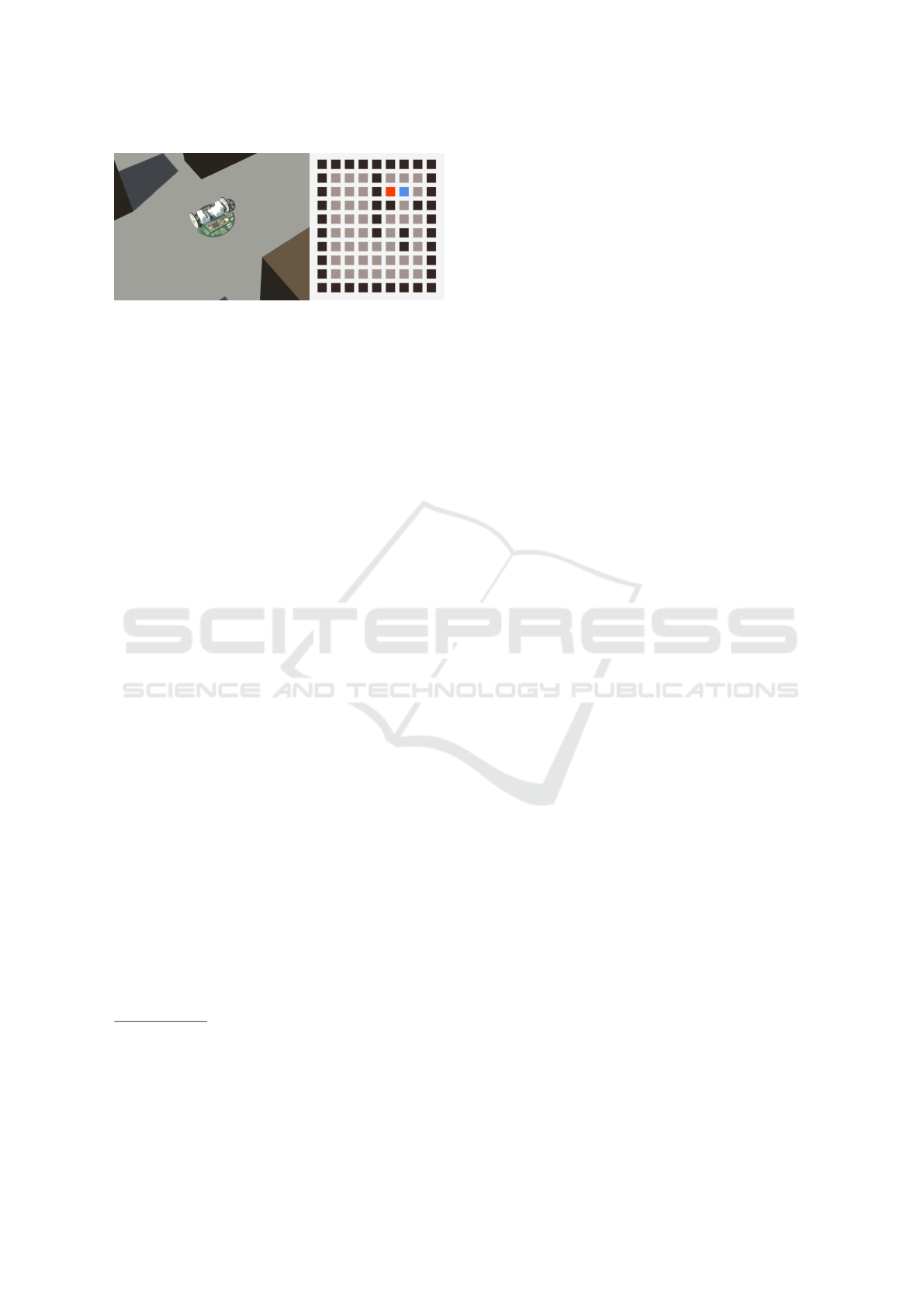
Figure 1: Left: An agent moving in continuous space in

MAES. Right: a traditional grid based simulation.

lares and Chaimowicz, 2016), and Random Ballistic

Walk (RBW) from (Kegeleirs et al., 2019), the latter

being used as a baseline for the comparisons.

Section 3 delves into the mapping of the algo-

rithms onto a continuous space, and other design de-

cisions needed to map the algorithms on a common

comparison framework.

Section 4 describes the MAES tool

, which was

developed to demonstrate our approach. It is based

on the Unity physical engine (Unity Technologies,

2021), and allows to simulate the algorithms on build-

ing maps (B-Map) featuring hallways and rooms, and

cave maps (C-Map) full of irregular shapes. The tool

allows for visual inspection for easier debugging and

comparison of implemented algorithms, and draws

comparisons in terms of coverage and exploration,

which we deﬁne in Section 2.1.

Results of simulations performed on both B-map

and C-map are reported in Section 5, and Section 6

draws conclusions and proposes future work, both in

terms of extension of the MAES simulator, and re-

garding the application of our framework to more sce-

narios.

Summarizing, the main contributions of this paper

include:

• A mapping SSB, LVD and TNF to continuous

space and on common hardware capabilities (Sec-

tion 3)

• MAES, a simulation tool for testing algorithms in

continuous space and on common hardware capa-

bilities. (Section 4)

• A comparison of the performance of the mapped

algorithms in a realistic simulator. Since the algo-

rithms have different hardware requirements, this

also provides insight into the beneﬁt of extra hard-

ware capabilities. (Section 5)

A video demonstration of MAES can be

found at https://youtu.be/lgUNrTfJW5g. MAES is

open source and the source code can be found at

https://github.com/MalteZA/MAES.

2 BACKGROUND INFORMATION

This section prepares the scene for the rest of the pa-

per, by deﬁning a few key concepts formally, and de-

scribing and comparing the algorithms we focus on.

2.1 Deﬁnitions

Deﬁnition 1. A grid space G is a movement space

where for any given position x ∈ G, x ∈ (Z ×Z).

Movement in a grid space consists of discrete

steps from cell to cell. A step can only move an agent

from its current cell to one of its immediate neigh-

bours. There are four or eight possible movement

directions, depending on whether diagonal steps are

allowed.

Deﬁnition 2. A Continuous space C is a movement

space where for any given position x ∈ C , x ∈ (R×R)

In a Continupus space, if an agent moves a dis-

tance of d in any direction between time t

and t

it will passy by uncountably inﬁnitely many possible

positions x in that time range.

Deﬁnition 3. An agent’s physical body has an area

that covers (or ’shadows’) some movement space, and

Coverage describes the amount of accumulated area

that an agent’s body-area has physically covered dur-

ing the process of moving through a movement space.

Deﬁnition 4. An agent has a ﬁeld of view (FOV)

which covers (or ”shadows”) a circular area of the

movement space. Exploration describes the amount

of accumulated open area an agent’s FOV has cov-

ered during the process of moving through a move-

ment space.

Deﬁnition 5. Simultaneous localization and map-

ping (SLAM) is constructing and updating a map of

explored area in a movement space, while simultane-

ously keeping track of an agent’s position within it.

Deﬁnition 6. Environment tagging refers to leaving

information at some position in the environment, that

can be used for indirect communication with other

agents.

2.2 Algorithms

2.2.1 Random Ballistic Walk

Random walk describes a category of approaches

where agents randomly alternate between rotating and

moving straight ahead. Random Walks require that

the agents be able to detect collision, move straight

ahead and rotate in place. Some variations also re-

quire the ability to estimate how far they have trav-

elled since the previous rotation.

SDMIS 2022 - Special Session on Super Distributed and Multi-agent Intelligent Systems

528

In (Kegeleirs et al., 2019), several variations on

random walks are compared including Brownian mo-

tion, L

evy Walk, and RBW. In RBW, the straight

movement continues until the agent collides with ei-

ther an obstacle or another agent. According to

(Kegeleirs et al., 2019) RBW produce the best results

for coverage and mapping of unknown environments,

and thus RBW was selected as the baseline for the

comparison with more sophisticated algorithms.

2.2.2 Spiraling and Selective Backtracking

In the SSB (Gautam et al., 2018) algorithm, the agents

perform coverage by traversing sections of the map

following inward spiral patterns.

The SSB algorithm is designed for a grid space,

and movement is modelled as discrete steps between

cells. SSB also assumes that agents can communicate

globally. Finally, the algorithm design is rooted in the

assumption that agents are able to accurately build a

map of their environment and continually synchronize

this map across all agents. These two requirements

reduces the usability in real world scenarios.

In the SSB algorithm agents alternate between two

states: spiraling and backtracking. In the spiraling

state, agents follow a simple set of rules to traverse an

area in the pattern of an inward spiral. While spiral-

ing, the agents make note of neighbouring unexplored

cells as potential back-tracking points. Once spiraling

is completed the agent broadcasts its collected back-

tracking points to all other agents. Then, the agent

determines which backtracking point to choose as its

target by performing an auction where agents bid on

available backtracking points. Each agent calculates a

bid based on its distance from the backtracking point.

If an agent is in spiraling mode during an auction, its

bid values will also depend on the estimated number

of steps required to ﬁnish the ongoing spiral. If the

agents wins a backtracking point, it will travel to that

point and then begin the spiraling phase again. If the

agent does not win any backtracking points it will still

travel to the closest candidate to avoid being idle.

2.2.3 Local Voronoi Decomposition

The idea behind LVD (Fu et al., 2009) is to achieve

task allocation using only indirect communication in

the form of the position of visible agents and obsta-

cles.

Each agent computes Voronoi regions from the ar-

eas of the map within line of sight (usually 360 de-

grees around the agent) at a given time, using other

agents’ location and walls/obstacles within line of

sight. The visibility range is not mentioned in the

original paper, but the illustrations in (Fu et al., 2009)

seem to indicate that it is inﬁnite, so we will in this

paper assume inﬁnite visibility range for LVD.

In LVD, an occlusion point is deﬁned as a corner

or obstacle where the line of sight is broken. All LVD

agents employ local SLAM to detect areas that they

have themselves previously covered, as well as previ-

ously covered occlusion points.

Pseudo code of the LVD algorithm can be seen in

Listings 1 and 2. The agents see the map as a grid

of tiles, which are explored when an agent has visited

. A tile can be within view but not explored yet.

Listing 1: LVD Algorithm 1 - Divide and Conquer.

1 // Divide part

2 For each cell in view

3 if the cell is closer to agent than to other agents

4 mark the cell as within region

5 end if

6 end for

7 // Conquer part

8 if there is just one unexplored cell within region

9 move to it

10 else if there are more than one unexplored cell

11 move in an ordered list, e.g. [North, East, South, West]

12 else

13 Enter Search Mode

14 end if

15 go to 1

Listing 2: LVD Algorithm 2 - Search Mode.

1 // Consider all occlusion points within view.

2 if at any time an unexplored cell appears within region then

3 exit Search Mode and go back to Algorithm 1

4 end if

5 if there is at least one occlusion point which has not been

visited during the Search Mode→

6 move to the nearest occlusion point which has not been

visited→

7 else if all occlusion points have already been visited

8 move to the least recently visited occlusion point

9 else if there are no occlusion points or if the only occlusion

point has just been visited→

10 move to the nearest Voronoi boundary which does not

11 coincide with any obstacle

12 end if

In its Divide and Conquer Mode, the algorithm

considers that agents sense other agents close by and

then use this information to divide the currently visi-

ble tiles into Voronoi regions, i.e. always delegating

a given tile to the agent closest to it. Each division

is computed independently by the agent. If any tiles

within a given agent’s Voronoi region are unexplored,

the agent will move to them in a conﬁgurable order,

e.g. ﬁrst north, then east, south and west. If no tile is

unexplored, the agent enters the Search Mode.

In the Search Mode the agent considers occlusion

points within line of sight, and it moves to an occlu-

Thus, LVN deﬁnition of explored correspond to what

this paper deﬁnes as covered.

Comparison of Online Exploration and Coverage Algorithms in Continuous Space

529

sion point that is likely to lead to an area with unex-

plored tiles. If all occlusion points have been visited

during the current phase of Search Mode, the agent

moves to the least recently visited one. If no occlusion

point is within line of sight, or they have all been vi-

sited recently, the agent moves to the nearest Voronoi

boundary which does not coincide with an obstacle,

in order to search for new unexplored tiles, while also

possibly ”pushing” other agents further out and away

from the already explored area. If at any time during

the Search Mode an unexplored tile comes into line of

sight, the agent exits Search Mode and returns to the

Divide and Conquer Mode.

2.2.4 The Next Frontier

TNF (Colares and Chaimowicz, 2016) is a frontier-

based exploration algorithm that works by detecting

and moving to boundaries between explored and un-

explored areas (frontiers). TNF prioritizes frontiers

through a combination of factors that are combined in

a utility function

U( f ) = Inf( f ) + Dist( f ) − Coord( f ) (1)

where f is a frontier, Inf( f ) is an Information Fac-

tor (prefer higher concentrations of cells of interest),

Dist( f ) is a Distance Factor (prefer frontiers at a cer-

tain conﬁgurable distance away), and Coord( f ) is a

Coordination Factor (dismiss frontiers that are close

to other agents). TNF agents can detect and map out

the local environment through SLAM, and can merge

maps with other agents when they are within commu-

nication distance. The TNF paper does not mention

any speciﬁc range requirements in regard to commu-

nication and area detection.

The Information Factor is used to prioritize cells

that are likely to contribute more valuable informa-

tion by being explored. An uncertain cell sitting in a

large concentration of other uncertain cells in a fron-

tier should be more valuable to explore than a single

uncertain cell in a completely discovered area. A cells

occupancy-value is seen as a number between 0 and

1, where 0 is a free cell, 0.5 an unexplored cell and

1 an occupied cell, and the cell’s contribution to the

Information Factor is modeled as a non-normalized

Gaussian function centered on 0.5. The Information

Factor of a frontier f can then be calculated as

Inf( f ) =

∑

c∈ f

G(c) +

∑

∈N

G(n

)

(2)

where G is the Gaussian function mentioned previ-

ously, N is all neighbours of cell c, and n

is the i

neighbour of c.

The Distance Factor is based on the idea that an

agent might prefer to prioritize frontiers at a certain

distance over others. The distance of a frontier is

calculated using what is referred to as a ”wavefront”,

starting from the position of the agent going towards

the frontier. This distance is then normalized to a

value (a real number) between [0..1], and the ﬁnal

Distance Factor is calculated as

Dist( f ) = wavefront( f )

α−1

× (1 − wavefront( f ))

β−1

(3)

where α and β are the conﬁguration parameters used

to control at which distance a frontier is favored. The

TNF authors found the most promising results using

the conﬁgurations (α = 3, β = 9), (α = 5, β = 9), or (α =

8, β = 8).

The Coordination Factor is the ﬁnal part of the

Utility Function, where an agent will prefer to explore

frontiers that are relatively far away from neighbour-

ing agents. Once again, a Wavefront Function is used,

but this time the starting position is of a neighbouring

agent, and this Coordication Factor is calculated for

each neighbour the agent can see at the time of calcu-

lation.

2.2.5 Requirements Summary

Table 1 lists the agent capability requirements for

each of the algorithms. The Environment Tagging and

SLAM criteria for LVD are parenthesized because the

functionality required by LVD can be achieved using

either one, as described in subsection 2.2.3.

Table 1: Requirements for each algorithm.

Collision Det.

Object Det.

Env. tagging

SLAM

Distri. SLAM

Local Com.

Global Com.

RBW 3

LVD 3 3 (3) (3)

TNF 3 3 3 3 3

SSB 3 3 3 3 3 3

2.3 Related Work

The simulation of multiple agent coverage algorithms

in realistic simulation settings is a relatively unex-

plored research area. Only few papers can be found

in the bibliography on this topic.

In (Gautam et al., 2018) a comparison of cov-

erage performance is provided for existing algo-

rithms with reduced communication range. This

paper compares SSB, Multiple-Depth-First-Search

(MDFS), Brick & Mortar (BNM), Boustrophedon and

backtracking mechanism (BOB) and Backtracking

SDMIS 2022 - Special Session on Super Distributed and Multi-agent Intelligent Systems

530

Spiral Approach - Cooperative Multi Robot (BSA-

CM). SSB achieved the best results. The comparison

is, however, performed in a grid base simulation us-

ing only two different maps - a basic and a Cluttered

map.

In (Gautam et al., 2021), SSB, BOB, and BSA-

CM are compared with different communication

range restrictions and number of agents. The algo-

rithms are compared in terms of coverage and redun-

dant coverage using hardware FireBird V robots on

a small plane. SSB and BSA-CM performs similarly

and better than BOB in terms of avoiding redundant

coverage.

3 MAPPING TO CONTINUOUS

SPACE

LVD and SSB operate in a grid space, where the cell

size is roughly equal to the size of the agent, and this

section describes a mapping from continuous space

to grid space for them. Moreover, other issue can ap-

pear when mapping the algorithm to a more realistic

framework, such as by considering that agent can ac-

tually collide with each other. Finally, TNF leaves

some design parameters to be deﬁned , and this sec-

tion takes care of this detail too.

Both LVD and SSB use SLAM, and the mapping

can be implemented by overlaying a grid on top of

their environment map in the Continuous Space. Each

tile in the overlay is considered either open or solid,

with the entire tile considered solid if any part of a

solid object is detected within the bounds of the tile.

For SSB, this grid overlay and accompanying tile sta-

tuses are synchronized along with the map itself.

The above approach limits maneuverability, as

otherwise traversable areas may be marked as solid,

depending on the alignment of the grid. An illustra-

tion of this problem can be seen in Figure 2 where

(a) shows the environment map constructed by an

agent. The agent could comfortably ﬁt through both

the west and east openings. However, as illustrated

in (b), the alignment of the grid can change perceived

traversability of the openings, if the tiles are too big.

To guarantee that the grid will always provide an

opening through a passage, the passage must be at

least as wide two tiles, as illustrated in (c). Similarly,

to guarantee open tiles in diagonal passages, the pas-

sages must be at least twice as wide as the diagonal of

a tile. This approach also reduces the area that will be

covered, as some free area will be perceived as solid

by the agent, thus not needed to be covered.

Figure 2: Illustration of grid overlay. (a) An agent (red) in a

Continuous Space with obstacles (black). (b) A grid overlay

with large tiles. Red tiles are perceived as solid and grey

tiles as traversable. (c) A more ﬁne grained grid overlay.

3.1 Selective Spiraling and

Backtracking

SSB is built upon an algorithm called BSA-CM (Gon-

zalez and Gerlein, 2009b). Apart from the aforemen-

tioned grid mapping approach, BSA-CM assumes

collision avoidance to be trivial, as all agents can

move at the same time in discrete steps between cells.

In our simulation, on the other hand, coordination and

timing issues arise, as an agent may partially occupy

up to four cells at the same time. To avoid collisions,

we introduce a tile reservation system, where agents

will secure a reservation for a tile before moving

into it. Reservation requests are broadcast to nearby

agents, and after a time delay, the reservation is as-

sumed to be accepted. To avoid delaying movement

unnecessarily while waiting for reservations, agents

in our implementation will attempt to predict their

path, and reserve several tiles in advance.

Multiple agents may attempt to reserve the same

tile at the same time, in which case the conﬂict is

resolved by accepting the reservation from the agent

with the highest id.

3.2 Local Voronoi Decomposition

The mapping of LVD to continuous space leads to a

series of challenges, which are not present in the orig-

inal paper since it uses Grid Space.

3.2.1 Empty Voronoi Regions

In a grid, an agent’s Voronoi region will never be

empty in terms of tiles, since the tile on which

the agent stands is always contained in the agent’s

Voronoi region. In continuous space, however, an

agent can be positioned in-between other agent that

are closer to the center of tiles and thus own them, see

Figure 3. We solved this issue by having the center

agent stay idle, since the surrounding agents will have

their respective Voronoi regions reach out from each

of the four corners and thus eventually move away

and set the center agent free.

Comparison of Online Exploration and Coverage Algorithms in Continuous Space

531

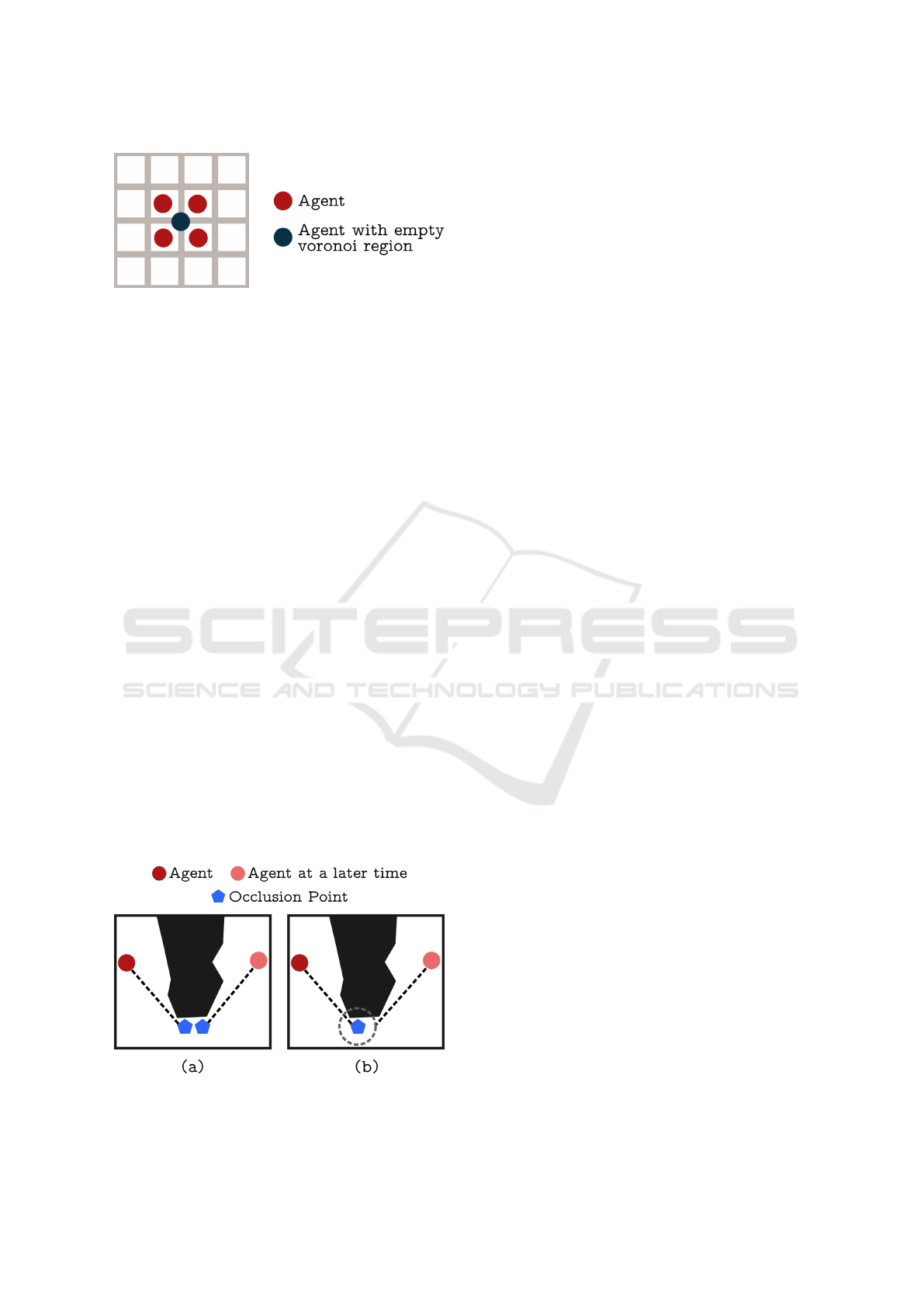
Figure 3: Illustration of an agent with an empty voronoi

region.

3.2.2 Calculation Interval

In LVD the agents move in a grid using discrete move-

ment, and recalculate the Voronoi regions after ev-

ery discrete move. However, this is not possible in

continuous space, as a change in position may be in-

ﬁnitesimally small. This begs the question of when to

recalculate Voronoi regions and ﬁnd the next task to

complete. We decided that an agent would recalculate

whenever it collides with anything, or if it reaches the

tile it was heading for.

Additionally, LVD mandates, that an agent should

exit Search Mode whenever an unexplored tile comes

into line of sight. It would be unfeasible to look for

unexplored tiles at every inﬁnitesimally small step

of movement. We decided to recalculate periodi-

cally at a given interval, even if they have not col-

lided or reached their current target. The interval is

shorter while in Search Mode to make it likely that

the agent exits Search Mode as soon as an unexplored

tile comes into line of sight.

3.2.3 Occlusion Points with Multiple Visits

In Search Mode the agent ﬁrst explores all occlusion

points within line of sight. In continuous space with a

high resolution slam map it can, however, be difﬁcult

to keep track of which occlusion points have been vi-

sited. When visiting occlusion points, the agent heads

Figure 4: (a) An agent identifying the same occlusion point

as two distinct points (b) Two points are considered the

same point, and the agent will not revisit the occlusion point

for the closest occlusion point it sees, which can how-

ever result in multiple visits to the same occlusion

points. Consider Figure 4(a), where the agent sees

an occlusion point and thus moves to this point and

around the obstacle. Now, however, the agent sees the

same occlusion point but from a different perspective.

Due to the shape of the obstacle the previous occlu-

sion now appears to be a new occlusion point, since

it is slightly offset to the right. This causes the agent

to revisit an already visited occlusion point. In order

to avoid this issue, we consider all occlusion points

within some distance of each other to be the same (see

Figure 4(b)).

3.3 The Next Frontier

TNF was originally designed to operate in a continu-

ous space. As mentioned in Section 2.2.4, TNF sees

the environment as a set of cells, where the boundaries

between the fully explored cells and the unknown

cells make up the frontiers to move to. However, a

design decision is required regarding how to imple-

ment the components of the Utility Function.

In order to prioritize cells where an agent is the

least certain of the cell’s state (i.e. cells with an In-

formation Factor contribution close to 0.5), the au-

thors of (Colares and Chaimowicz, 2016) made use of

a non-normalized Gaussian function centered around

0.5. However, the authors only mention the center

of the function’s peak, and do not specify its height

nor its deviation. For our implementation, we assume

a function peak of 5 and a deviation of 0.1, as this

seems to produce a usable behavior.

With regards to the Distance Factor, the TNF au-

thors mention the use of a wavefront function to mea-

sure the distance from an agents position to the cells

of a frontier, without providing much details on how

to build it. For our implementation, we assume eu-

clidean distance (L

norm) to each of the cells, as this

is consistent with how a wavefront is depicted in the

paper. With regards to the normalization of the dis-

tances to the frontiers to values between [0, 1], we as-

sume that a wavefront is normalised by identifying

the most distant cell’s distance D

MAX

, and dividing

the distance of every other cell by D

MAX

. As men-

tioned in Section 2.2.4, the ﬁnal Distance Factor value

is conﬁgurable with the variables α and β. For this

implementation, we chose to use one of the authors’

suggested conﬁguration of (α = 8, β = 8).

We implemented the Coordination Factor by sum-

ming up the results for each neighbouring agent.

We acknowledge that other approach might be vi-

able, for example dividing each wavefront distance

by the number of known neighbours. Finally, to take

SDMIS 2022 - Special Session on Super Distributed and Multi-agent Intelligent Systems

532

into consideration collisions between two (or more)

agents, we use a mitigation-procedure that implies

that, after a collision, each agent looks in its imme-

diate surroundings, and go to a location that is free

and not occupied by another agent.

4 THE MAES TOOL

This section describes the MAES tool, which we de-

veloped for conducting the experiments shown in Sec-

tion 5. MAES is a deterministic 2D discrete time-

step physics-based simulation, visualized in 3D. The

simulator uses the Unity Engine (Unity Technolo-

gies, 2021), for visualization and physics simulation.

Physics are simulated at a rate of 100 ticks per simu-

lated second. The reaction time of the agent, i.e. how

often the agents apply their exploration algorithms to

the current data, is 10 ticks.

MAES features a map generator than can gener-

ate two types of maps, i.e. the cave map type (C-

Map) and the Building map type (B-Map). MAES

provides an agent control interface that allows im-

plementation of exploration algorithms. This inter-

face provides access to movement controls, commu-

nication, object detection and SLAM. MAES allows

many of its feature to be conﬁgured, and it takes

parameters for agent constraints, for physics simu-

lation, and for map generation. A list of all pos-

sible parameters for the simulator can be seen on

https://github.com/MalteZA/MAES, where the code

is made available to the public.

4.1 Environment Maps

In order to study useful settings, MAES generates ran-

dom maps ﬁtting the characteristics of B-maps and C-

maps.

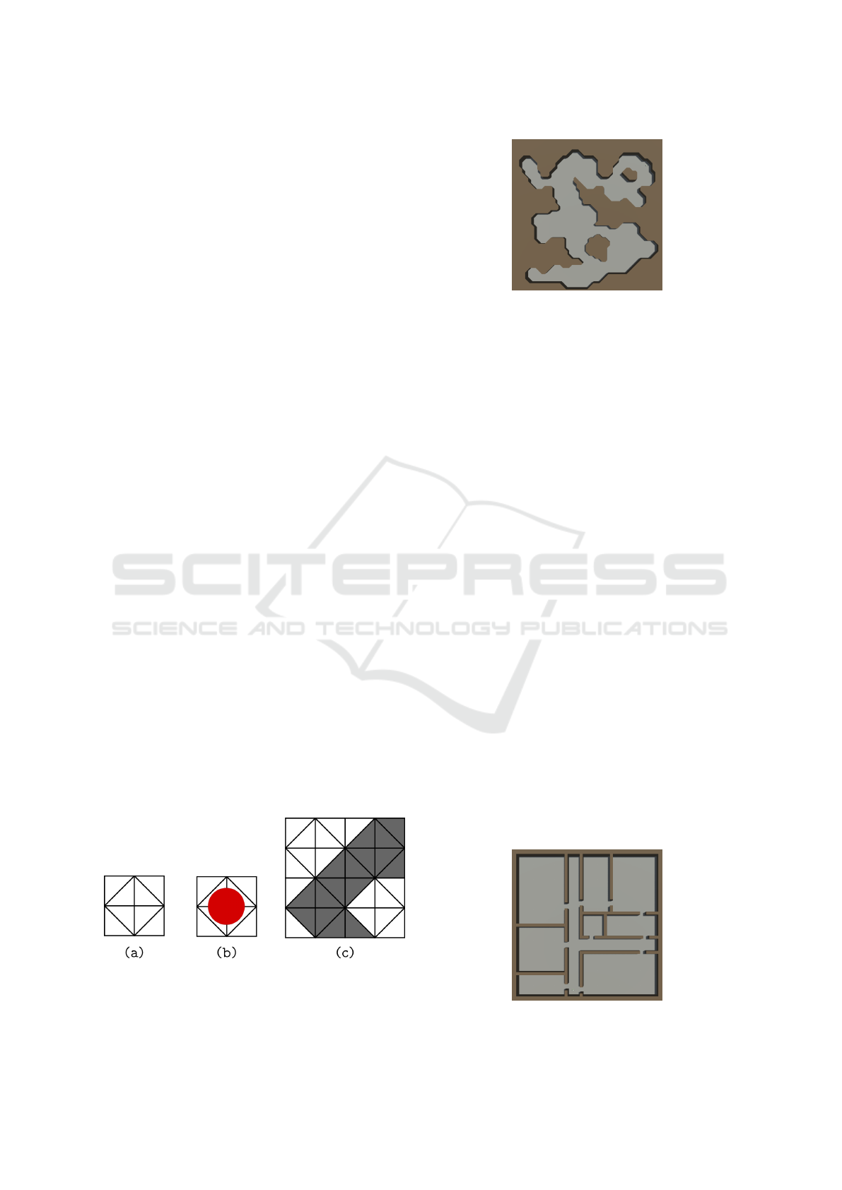
A map consists of a number of tiles, where each

tile consists of 8 triangles arranged, as shown in Fig-

ure 5(a). An agent can be up to as big as a tile. In Fig-

Figure 5: The tile structure of the map. (a) The arrangement

of the of 8 triangles forming a single tile. (b) The size of an

agent relative to tile. (c) Four tiles, where solid triangles

form an obstacle.

Figure 6: An example of a 50x50 generated cave map.

ure 5(b) an agent with size 0.6 times a tile is shown.

Finally, each triangle may be open or solid, where

open tiles are freely traversable and solid triangles are

impassable. Obstacles with complex shapes can be

formed by chaining solid triangles as shown in 5(c).

4.1.1 Cave Map Type

The C-map type is relevant for example for the use

cases of exploration and search & rescue in an irregu-

larly shaped environment. The C-map generator starts

by randomly distributing wall and room type cells in a

grid of a given size. It then uses neighbour smoothing,

based on rules similar to Conway’s Game of Life, to

create sections of walls and rooms, e.g. a tile with 4 or

more solid neighbour tiles will turn solid and the other

way around. Now the generator can interconnect all

rooms (groups of open tiles) created while ensuring

that every part of the cave is reachable from every

other part. In order to make the cave more realistic

and irregular we use the Marching Squares algorithm

to round off edges. An example image of a C-map

can be seen in Figure 6.

4.1.2 Building Map Type

The B-map type is relevant for simulating use cases

such as ﬂoor cleaning and search & rescue in build-

ings. The generated maps are made to look like the

ﬂoor plan of a building. The B-map generator creates

a grid of a given size and marks each cell as being

either wall, hallway or room. The generator starts by

Figure 7: An example of a 50x50 generated building map.

Comparison of Online Exploration and Coverage Algorithms in Continuous Space

533

Figure 8: The 3D model of the MONA-inspired agent used

in MAES.

connecting all the hallways, then it recursively splits

the spaces between to hallways to create rooms, with

room size deﬁned at random. Finally all the rooms are

connected to each other with doors in such a way that

all rooms are reachable from the hallways. Figure 7

shows an example of a B-map.

4.2 Agents

Within MAES, an agent’s capabilities can vary de-

pending on the parameters that describe the simula-

tion at hand, e.g. limited vision, broadcasting range

etc. An image of the 3D model of an agent, inspired

by the MONA robots (Arvin et al., 2019), can be seen

in Figure 8.

4.2.1 Movement

An agent is able to rotate in place and moving straight

ahead, and the agent is not able to rotate while moving

forwards. Movement is simulated through the Unity

2D Physics Engine by applying force at the position

of each wheel. This simulation accounts for inertia,

drag, and collisions with obstacles and other agents.

The agents of the MAES simulator can reach a top

speed of 3 tiles / second (or 10 logic ticks). The tile

size can vary depending on the scale of the map. We

decided that the agent takes about 30 physics ticks to

reach its top speed. Drag is a function of speed, which

in combination with inertia results in non-constant ac-

celeration, leading to an agent reaching half its top

speed (about 1.5 tiles / second) after just 4 ticks.

4.2.2 Sensors and Communication

Agents are able to sense other agents at a given dis-

tance, which is a simulation parameter. In order to ac-

commodate variety of scenarios with differing hard-

ware capabilities, the signal sensing other agents can

also be conﬁgured to be blocked by walls, i.e. requir-

ing line of sight. Agents detect collisions with walls

and with other agents, and can detect a nearby wall

and the angle to said wall. This could for example

be achieved using a LIDAR scanner in the real world.

Agents can communicate through broadcasting, and

both communication range and the capabilities to pass

walls is deﬁned via simulation parameters. Line of

sight is determined using ray tracing. Beyond line of

sight and maximum range, no other signal loss is sim-

ulated.

Finally, agents can drop tags on the ground to de-

posit information in the environment and communi-

cate indirectly with other agents, as required for ex-

ample by LVD (Section 2.2.3). Tags can only be

dropped at an agent’s current position, but data can

be written to and read from at a conﬁgurable distance.

4.2.3 Simulated SLAM

If enabled, the agent can provide an environment map

generated via SLAM to the algorithm being simu-

lated. SLAM is simulated by performing a series of

ray traces from the position of the agent, and measur-

ing the distance that the rays traveled before collid-

ing. This emulates the behavior of technologies such

as LIDAR scanners.

The agent continuously constructs a ”SLAM map”

using the ray tracing information when it becomes

available. If any object is detected within the region

of a tile, then that entire tile is marked as solid. If a

ray trace is sent in the direction of a tile, and no ob-

ject is found, the tile is assumed to be open, unless

previous traces indicate that it is solid. The agent has

access to an approximation of its location within the

SLAM map. The simulation can be conﬁgured to au-

tomatically synchronize SLAM maps of agents that

are within communication range of each other.

4.2.4 Interfaces

MAES is intended to support the implementation of

many different algorithms. For this reason we expose

an interface for the algorithms to control the agents

and provide access to sensor information. The in-

terface is created to allow for implementing all of

the hardware requirements mentioned in Table 1, e.g.

SLAM map, environment tagging, etc.

4.3 Debugging Features

As MAES should function as a testbed for many dif-

ferent algorithms we include a wide variety of debug-

ging tools. A menu is included for controlling the

camera view over the simulation, as well as changing

the simulation speed. Additionally, agents can be in-

dividually selected, which makes the camera follow

SDMIS 2022 - Special Session on Super Distributed and Multi-agent Intelligent Systems

534

the agent as well as reveal debugging information in

a side bar regarding the selected agent.

Furthermore, slam maps, communication, and en-

vironment tagging can be visualized. When a simula-

tion is running the surface of the map is highlighted

in green if any agent at any point has explored it. If an

agent is selected, the surface reveals in blue the tiles

included in the slam map for said agent. The slam

map can also include sections of the map revealed by

other agents, if slam synchronization is enabled and

the two agents have been within communication dis-

tance of each other. Environment tagging is visualised

using colored boxes on the ground where an agent has

tagged the environment.

5 EXPERIMENTS AND RESULTS

For quantifying performance we use two metrics:

coverage and exploration, explained in Deﬁnition 3

and Deﬁnition 4 respectively. The coverage metric is

important for purposes like robotic lawn mowers and

cleaning robots such as autonomous vacuum clean-

ers, where the robots need to efﬁciently and precisely

cover areas. The exploration metric is important for

agents when exploring an area to generate a navigable

map of the environment, or in search & rescue scenar-

ios where it is vital to quickly explore large areas.

As described in Section 4.1 a MAES map consists

of tiles, where each tile consists of 8 triangles. Ex-

ploration is measured in triangles, and a triangle is

considered to be explored when an agent’s simulated

Lidar trace has intersected with the triangle. Cover-

age is measured in whole tiles, and a tile is considered

covered once the center point of an agent has entered

the bounds of the tile.

For both B-map and C-map, in order to test the

scalability of the algorithms, we simulated different

map sizes, namely 50x50, 100x100 and 200x200. We

used an agent size of 0.6 tiles. We run each algorithm

20 times for 60 simulated minutes, each with a differ-

ent random seed, leading to different maps. If an al-

gorithm reaches a coverage of 99.5% (or TNF reaches

an exploration of 99.5%), the simulation ends before

the 60 minute mark. Each algorithm has its own agent

constraints as showed on Table 1. For example, SSB

assumes global communication, while LVD does not

need direct communication at all.

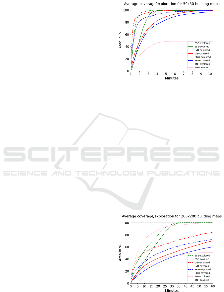
5.1 Building Scenario

According to Figure 9, LVD leads in exploration for

the ﬁrst few minutes after which SSB takes the lead

Figure 9: Comparison of algorithm performance in terms of

exploration and coverage for the building type map of size

50x50. Average results of 20 random seeds.

in the C-map with a size of 50x50. In terms of cov-

erage, SSB performs the best and has the map fully

covered on average after about 5 minutes. RBW and

LVD achieve similar coverage with a slight advantage

to LVD.

Figure 10 shows the results for the 200x200 map

can be seen. Here TNF achieves the best result in

terms of early exploration. SSB, however, eclipses the

exploration performance of TNF after about 30 min-

utes. LVD and RBW are signiﬁcantly behind on ex-

ploration and neither manages to ﬁnish within 60 min-

utes. LVD achieves a slightly better result than RBW

in terms of exploration. SSB achieves the fastest cov-

erage and ﬁnishes on average after about 37 minutes.

RBW and LVD reaches about 56% and 64% coverage

respectively after 60 minutes.

We omit the results for 100x100 B-maps, since

they were intermediate between the 50x50 and the

200x200 B-maps.

Figure 10: Comparison of algorithm performance in terms

of exploration and coverage for the building type map of

size 200x200. Average results of 20 random seeds.

Comparison of Online Exploration and Coverage Algorithms in Continuous Space

535

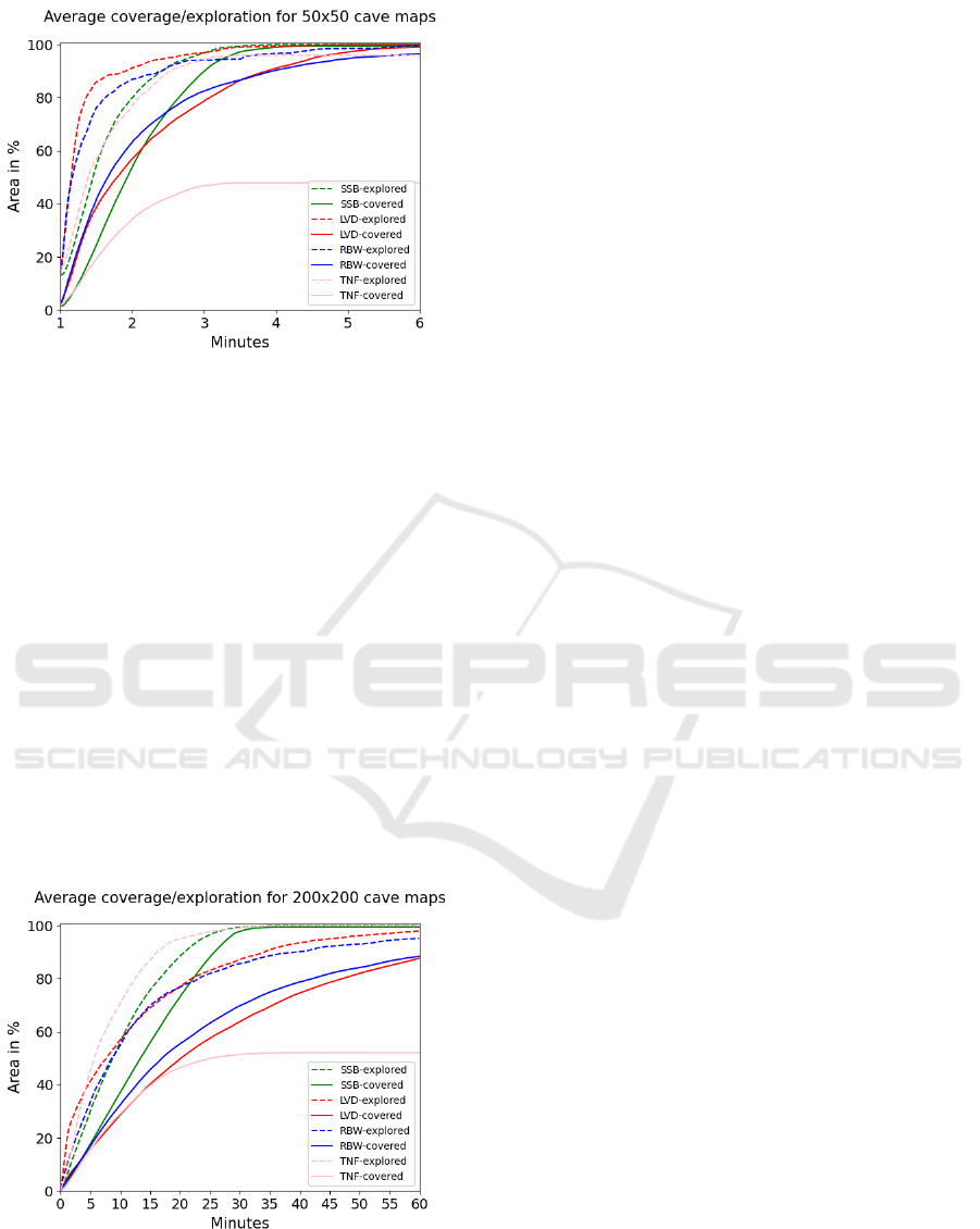
Figure 11: Comparison of algorithm performance in terms

of exploration and coverage for the cave type map of size

50x50. Average results of 20 random seeds.

5.2 Cave Scenario

In Figure 11 it can be seen, that LVD explores the

fastest, followed by RBW and then TNF and SSB. In

terms of coverage SSB is slightly faster with RBW

and LVD both ﬁnishing last after about 6.5 minutes.

The results for the 200x200 C-map, seen on Fig-

ure 12, has TNF exploring the map the fastest, fol-

lowed by SSB. LVD and RBW achieves similar ex-

ploration rates. SSB covers the larger map signiﬁ-

cantly faster than the other algorithms. Neither RBW

nor LVD ﬁnishes the coverage within the 60 minutes

of the simulation. RBW and LVW both manage about

83% coverage.

We omit the results for 100x100 C-maps, since

they were intermediate between the 50x50 and the

200x200 C-maps.

Figure 12: Comparison of algorithm performance in terms

of exploration and coverage for the cave type map of size

200x200. Average results of 20 random seeds.

6 CONCLUSIONS AND FUTURE

WORK

The paper proposes a continuous space mapping for

the SSB, LVD and TNF algorithms, and presents the

open source simulation tool MAES, which can be

used for developing and evaluating exploration algo-

rithms in a continuous 2D space. The mapped algo-

rithms were implemented and compared statistically

through repeated runs with randomly generated maps.

RBW was implemented as a baseline for comparison

with other the algorithms.

In terms of coverage, SSB performed signiﬁcantly

better than the other algorithms in both B-map and C-

map types. This performance comes at the cost of

reduced realism, as SSB assumes global communica-

tion and distributed SLAM capabilities.

TNF shows good results for exploration, exceed-

ing other algorithms in large maps for both B-map

and C-map types. TNF does, however, also require

distributed SLAM to operate.

LVD achieves slightly better results in terms of

coverage and exploration in most maps than RBW

while only using strictly local information.

Future work will consider to implement more

state-of-the-art algorithms, and propose algorithms

tailored on the realistic framework we propose. More-

over, there are aspects of the algorithms that can be

further studied such as scalability with respect to the

number of agents, and the effect of lower visibil-

ity and transmission ranges. Finally, the MAES tool

can beneﬁt from more development, such as to allow

for batch (no UI) and distributed simulations for en-

hanced performance.

ACKNOWLEDGEMENTS

This work was partly founded by the TECH fac-

ulty project “Digital Technologies for Industry 4.0”,

Aalborg University, and by the Villum Investigator

Project ”S4OS: Scalable analysis and Synthesis of

Safe, Small, Secure and Optimal Strategies for Cyber-

Physical Systems”.

REFERENCES

Agmon, N., Hazon, N., and Kaminka, G. A. (2008). The

giving tree: constructing trees for efﬁcient ofﬂine and

online multi-robot coverage. Annals of Mathematics

and Artiﬁcial Intelligence, 52(2):143–168.

Albani, D., Manoni, T., Arik, A., Nardi, D., and Trianni,

V. (2019). Field coverage for weed mapping: toward

SDMIS 2022 - Special Session on Super Distributed and Multi-agent Intelligent Systems

536

experiments with a uav swarm. In International Con-

ference on Bio-inspired Information and Communica-

tion, pages 132–146. Springer.

Arvin, F., Espinosa, J., Bird, B., West, A., Watson, S., and

Lennox, B. (2019). Mona: an affordable open-source

mobile robot for education and research. Journal of

Intelligent & Robotic Systems, 94(3):761–775.

Brambilla, M., Ferrante, E., Birattari, M., and Dorigo, M.

(2013). Swarm robotics: a review from the swarm

engineering perspective. Swarm Intelligence, 7(1):1–

41.

Cheraghi, A. R., Abdelgalil, A., and Grafﬁ, K. (2020). Uni-

versal 2-dimensional terrain marking for autonomous

robot swarms. In 2020 5th Asia-Paciﬁc Conference

on Intelligent Robot Systems (ACIRS), pages 24–32.

IEEE.

Colares, R. G. and Chaimowicz, L. (2016). The next fron-

tier: Combining information gain and distance cost for

decentralized multi-robot exploration. In Proceedings

of the 31st Annual ACM Symposium on Applied Com-

puting, SAC ’16, page 268–274, New York, NY, USA.

Association for Computing Machinery.

Fu, J. G. M., Bandyopadhyay, T., and Ang, M. H. (2009).

Local voronoi decomposition for multi-agent task al-

location. In 2009 IEEE International Conference on

Robotics and Automation, pages 1935–1940.

Gautam, A., Richhariya, A., Shekhawat, V. S., and Mohan,

S. (2018). Experimental evaluation of multi-robot on-

line terrain coverage approach. In 2018 IEEE Interna-

tional Conference on Robotics and Biomimetics (RO-

BIO), pages 1183–1189.

Gautam, A., Soni, A., Singh Shekhawat, V., and Mohan,

S. (2021). Multi-robot online terrain coverage un-

der communication range restrictions – an empirical

study. In 2021 IEEE 17th International Conference on

Automation Science and Engineering (CASE), pages

1862–1869.

Gonzalez, E. and Gerlein, E. (2009a). Bsa-cm: A multi-

robot coverage algorithm. In 2009 IEEE/WIC/ACM

International Joint Conference on Web Intelligence

and Intelligent Agent Technology, volume 2, pages

383–386. IEEE.

Gonzalez, E. and Gerlein, E. (2009b). Bsa-cm: A multi-

robot coverage algorithm. In 2009 IEEE/WIC/ACM

International Joint Conference on Web Intelligence

and Intelligent Agent Technology, volume 2, pages

383–386.

Kambayashi, Y., Ugajin, M., Sato, O., Tsujimura, Y., Ya-

machi, H., Takimoto, M., and Yamamoto, H. (2009).

Integrating ant colony clustering method to a multi-

robot system using mobile agents. Industrial Engi-

neering and Management Systems, 8(3):181–193.

Kegeleirs, M., Garz

on Ramos, D., and Birattari, M. (2019).

Random walk exploration for swarm mapping. In Al-

thoefer, K., Konstantinova, J., and Zhang, K., editors,

Towards Autonomous Robotic Systems, pages 211–

222, Cham. Springer International Publishing.

Kegeleirs, M., Grisetti, G., and Birattari, M. (2021). Swarm

slam: Challenges and perspectives. Frontiers in

Robotics and AI, 8:23.

Oikawa, R., Takimoto, M., and Kambayashi, Y. (2015).

Distributed formation control for swarm robots using

mobile agents. In 2015 IEEE 10th Jubilee Interna-

tional Symposium on Applied Computational Intelli-

gence and Informatics, pages 111–116. IEEE.

Schranz, M., Umlauft, M., Sende, M., and Elmenreich, W.

(2020). Swarm robotic behaviors and current applica-

tions. Frontiers in Robotics and AI, 7:36.

Unity Technologies (2021). Unity Real-Time Development

Platform | 3D, 2D VR & AR Engine. https://unity.

com/.

Comparison of Online Exploration and Coverage Algorithms in Continuous Space

537