iRNN: Integer-only Recurrent Neural Network

Eyy

ub Sari, Vanessa Courville and Vahid Partovi Nia

∗

Huawei Noah’s Ark Lab, Canada

Keywords:

Recurrent Neural Network, LSTM, Model Compression, Quantization, NLP, ASR.

Abstract:

Recurrent neural networks (RNN) are used in many real-world text and speech applications. They include

complex modules such as recurrence, exponential-based activation, gate interaction, unfoldable normalization,

bi-directional dependence, and attention. The interaction between these elements prevents running them

on integer-only operations without a signiﬁcant performance drop. Deploying RNNs that include layer

normalization and attention on integer-only arithmetic is still an open problem. We present a quantization-aware

training method for obtaining a highly accurate integer-only recurrent neural network (iRNN). Our approach

supports layer normalization, attention, and an adaptive piecewise linear approximation of activations (PWL),

to serve a wide range of RNNs on various applications. The proposed method is proven to work on RNN-

based language models and challenging automatic speech recognition, enabling AI applications on the edge.

Our iRNN maintains similar performance as its full-precision counterpart, their deployment on smartphones

improves the runtime performance by 2×, and reduces the model size by 4×.

1 INTRODUCTION

RNN (Rumelhart et al., 1986) architectures such as

LSTM Hochreiter and Schmidhuber (1997) or GRU

Cho et al. (2014) are the backbones of many down-

stream applications. RNNs now are part of large-scale

systems such as neural machine translation Chen et al.

(2018); Wang et al. (2019a) and on-device systems

such as Automatic Speech Recognition (ASR) He et al.

(2019). RNNs are still highly used architectures in

academia and industry, and their efﬁcient inference

requires more elaborated studies.

In many edge devices, the number of computing

cores is limited to a handful of computing units, in

which parallel-friendly transformer-based models lose

their advantage. There have been several studies in

quantizing transformers to adapt them for edge devices

but RNNs are largely ignored. Deploying RNN-based

chatbot, conversational agent, and ASR on edge de-

vices with limited memory and energy requires further

computational improvements. The 8-bit integer neural

networks quantization (Jacob et al., 2017) for convolu-

tional architectures (CNNs) is shown to be an almost

free lunch to tackle the memory, energy, and latency

costs, with a negligible accuracy drop (Krishnamoor-

thi, 2018).

Intuitively, quantizing RNNs is more challenging

∗

Corresponding author

because the errors introduced by quantization will

propagate in two directions, i) to the next layers, like

feedforward networks ii) across timesteps. Further-

more, RNN cells are computationally more complex;

they include several element-wise additions and mul-

tiplications. They also have different activation func-

tions that rely on the exponential function, such as

sigmoid and hyperbolic tangent (tanh).

Accurate fully-integer RNNs calls for a new cell

that is built using integer friendly operations. Our main

motivation is to enable integer-only inference of RNNs

on specialized edge AI computing hardware with no

ﬂoating-point units, so we constrained the new LSTM

cell to include only integer operations.

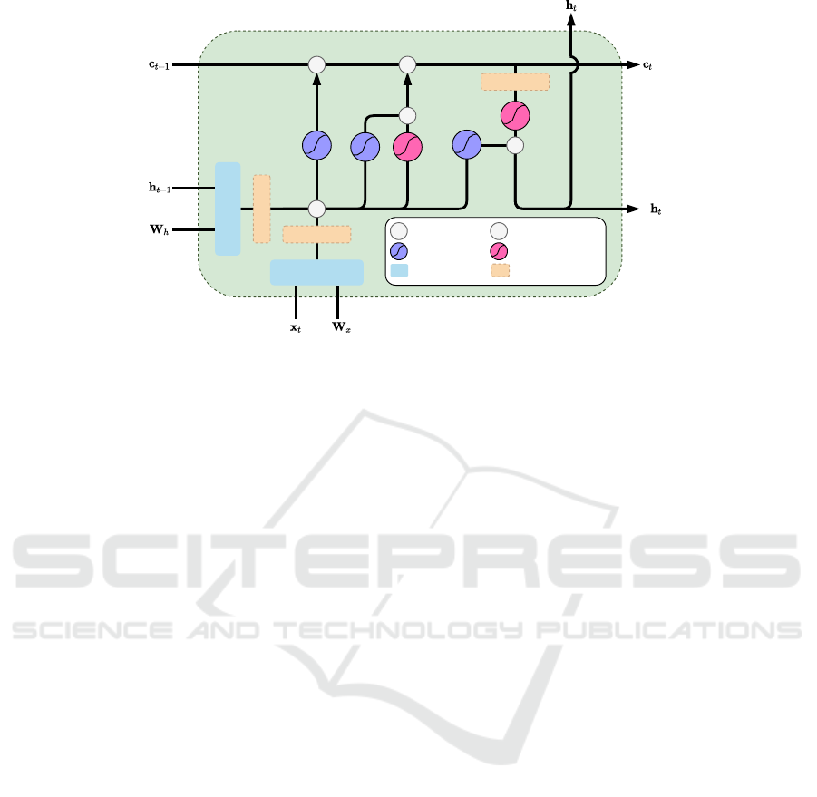
First we build a fully integer LSTM cell in which

its inference require integer-only computation units,

see Figure 1. Our method can be applied to any RNN

architecture, but here we focus on LSTM networks

which are the most commonly used RNNs.

Our contributions can be summarized as

•

providing a quantization-aware piecewise linear

approximation algorithm to replace exponential-

based activation functions (e.g. sigmoid and tanh)

with integer-friendly activation,

•

introducing an integer-friendly normalization layer

based on mean absolute deviation,

• proposing integer-only attention,

110

Sari, E., Courville, V. and Partovi Nia, V.

iRNN: Integer-only Recurrent Neural Network.

DOI: 10.5220/0010975700003122

In Proceedings of the 11th International Conference on Pattern Recognition Applications and Methods (ICPRAM 2022), pages 110-121

ISBN: 978-989-758-549-4; ISSN: 2184-4313

QMatmul

QMadNorm

QMatmul

QMadNorm

Quantized addition

Quantized sigmoid

PWL

Quantized multiplication

Quantized tanh PWL

Quantized matmul

Quantized MadNorm

(optional)

Figure 1: Example of an integer-only LSTM cell (iLSTM). Layer normalization change to quantized integer friendly MadNorm

(QMadNorm), full-precision matrix multiplications change to integer matrix multiplication (QMatmul), sigmoid and tanh

activations are replaced with their corresponding piecewise linear (PWL) approximations.

•

wrapping up these new modules into an LSTM cell

towards an integer-only LSTM cell.

We also implement our method on an anonymous

smartphone, effectively showing

2×

speedup and

4×

memory compression. It is the proof that our method

enables more RNN-based applications (e.g. ASR) on

edge devices.

2 RELATED WORK

With ever-expanding deep models, designing efﬁcient

neural networks enable wider adoption of deep learn-

ing in industry. Researchers recently started working

on developing various quantization methods (Jacob

et al., 2017; Hubara et al., 2018; Darabi et al., 2018;

Esser et al., 2020). Ott et al. (2016) explores low-bit

quantization of weights for RNNs. They show binariz-

ing weights lead to a massive accuracy drop, but ternar-

izing them keeps the model performance. Hubara et al.

(2018) demonstrate quantizing RNNs to extremely low

bits is challenging; they quantize weights and matrix

product to 4-bit, but other operations such as element-

wise pairwise and activations are computed in full-

precision. Hou et al. (2019) quantize LSTM weights

to 1-bit and 2-bit and show empirically that low-bit

quantized LSTMs suffer from exploding gradients.

Gradient explosion can be alleviated using normal-

ization layers and leads to successful training of low

bit weights Ardakani et al. (2018). Sari and Partovi Nia

(2020) studied the effect of normalization in low bit

networks theoretically, and proved that low-bit train-

ing without normalization operation is mathematically

impossible; their work demonstrates the fundamental

importance of involving normalization layers in quan-

tized networks. He et al. (2016) introduce Bit-RNN

and improve 1-bit and 2-bit RNNs quantization by con-

straining values within ﬁxed range carefully; they keep

activation computation and element-wise pairwise op-

erations in full-precision. Kapur et al. (2017) build

upon Bit-RNN and propose a low-bit RNN with mini-

mal performance drop, but they increase the number of

neurons to compensate for performance drop; they run

activation and pair-wise operations on full-precision

as well.

Wu et al. (2016) is a pioneering work in LSTM

quantization, which demonstrated speed-up inference

of large-scale LSTM models with limited performance

drop by partially quantizing RNN cells. Their pro-

posed method is tailored towards speciﬁc hardware.

They use 8-bit integer for matrix multiplications and

16-bit integer for tanh, sigmoid, and element-wise

operations but do no quantize attention Bluche et al.

(2020) propose an effective 8-bit integer-only LSTM

cell for Keyword Spotting application on microcon-

trollers. They enforce weights and activations to be

symmetric on ﬁxed ranges

[−4,4]

and

[−1,1]

. This

prior assumption about the network’s behaviour re-

strict generalizing their approach for wide range of

RNN models. They propose a look-up table of 256

slots to represent the quantized tanh and sigmoid acti-

vations. However, the look-up table memory require-

ment explodes for bigger bitwidth. Their solution

does not serve complex tasks such as automatic speech

recognition due to large look up table memory con-

sumption. While demonstrating strong results on Key-

word Spotting task, their assumptions on quantization

iRNN: Integer-only Recurrent Neural Network

111

range and bitwidth make their method task-speciﬁc.

3 BACKGROUND

We use the common linear algebra notation and use

plain symbols to denote scalar values, e.g.

x ∈ R

, bold

lower-case letters to denote vectors, e.g.

x ∈ R

, and

bold upper-case letters to denote matrices, e.g.

X ∈

m×n

. The element-wise multiplication is represented

by .

3.1 LSTM

We deﬁne an LSTM cell as













= W

+ W

t−1

, (1)

= σ(f

)  c

t−1

+ σ(i

)  tanh(j

), (2)

= σ(o

)  tanh(c

), (3)

where

σ(·)

is the sigmoid function;

is the input

hidden units dimension, and

is the state hidden

units dimension;

∈ R

is the input for the current

timestep

t ∈ {1, ...,T }

;

t−1

∈ R

is the hidden state

from the previous timestep and

is initialized with

zeros;

∈ R

4m×n

is the input to state weight ma-

trix;

∈ R

4m×m

is the state to state weight matrix;

} ∈ R

are the pre-activations to the

{

input,

forget, output

}

gates;

∈ R

is the pre-activation to

the cell candidate;

} ∈ R

are the cell state and

the hidden state for the current timestep, respectively.

We omit the biases for the sake of notation simplicity.

For a bidirectional LSTM (BiLSTM) the output hidden

state at timestep

is the concatenation of the forward

hidden state

−→

and the backward hidden state

←−

[

−→

;

←−

3.2 LayerNorm

Layer normalization Ba et al. (2016) standardizes in-

puts across the hidden units dimension with zero lo-

cation and unit scale. Given hidden units

x ∈ R

LayerNorm is deﬁned as

µ =

∑

i=1

, ˆx

= x

− µ (4)

std

∑

i=1

ˆx

, σ

std

(5)

LN(x)

= y

ˆx

std

(6)

where

(4) is the hidden unit mean,

ˆx

(4) is the

centered hidden unit

std

(5) is the hidden unit

variance, and

(6) is the normalized hidden unit. In

practice, one can scale

by a learnable parameter

or shift by a learnable parameter

. The LayerNormL-

STM cell is deﬁned as in Ba et al. (2016).

3.3 Attention

Attention is often used in encoder-decoder RNN ar-

chitectures (Bahdanau et al., 2015; Chorowski et al.,

2015; Wu et al., 2016). We employ Bahdanau atten-

tion, also called additive attention (Bahdanau et al.,

2015). The attention mechanism allows the decoder

network to attend to the variable-length output states

from the encoder based on their relevance to the cur-

rent decoder timestep. At each of its timesteps, the

decoder extracts information from the encoder’s states

and summarizes it as a context vector,

enc

∑

i=1

 h

enc

(7)

exp(e

)

∑

enc

j=1

exp(e

t j

)

(8)

= v

tanh(W

t−1

+ W

enc

) (9)

where

is the context at decoder timestep

which is

a weighted sum of the encoder hidden states outputs

enc

∈ R

enc

along encoder timesteps

i ∈ {1,...,T

enc

}

;

0 < α

< 1

are the attention weights attributed to each

encoder hidden states based on the alignments

∈ R

;

dec

and

enc

are respectively the decoder and en-

coder hidden state dimension;

∈ R

att

×m

dec

∈

att

×m

enc

}

are the weights matrices of output dimen-

sion

att

respectively applied to the query

t−1

and the

keys

enc

;

v ∈ R

att

is a learned weight vector. The

context vector is incorporated into the LSTM cell by

modifying (1) to













= W

+ W

t−1

+ W

(10)

where W

∈ R

dec

×m

enc

3.4 Quantization

Quantization is a process whereby an input set is

mapped to a lower resolution discrete set, called the

quantization set

. The mapping is either performed

from ﬂoating-points to integers (e.g. ﬂoat32 to int8)

or from a dense integer to another integer set with

lower cardinality, e.g. int32 to int8. We follow the

ICPRAM 2022 - 11th International Conference on Pattern Recognition Applications and Methods

112

Quantization-Aware Training (QAT) scheme described

in Jacob et al. (2017).

Given

x ∈ [x

min

max

]

, we deﬁne the quantization

process as

= q(x) =

+ Z

(11)

= r(x) = S

− Z

) (12)

max

− x

min

− 1

, Z

−x

min

(13)

where the input is clipped between

min

and

max

be-

forehand;

b.e

is the round-to-nearest function;

is the

scaling factor (also known as the step-size);

is the

bitwidth, e.g.

b = 8

for 8-bit quantization,

b = 16

for 16-bit quantization;

is the zero-point corre-

sponding to the quantized value of 0 (note that zero

should always be included in

min

max

]

);

q(x)

quan-

tize

to an integer number and

r(x)

gives the ﬂoating-

point value

q(x)

represents, i.e.

r(x) ≈ x

. We refer

min

max

,b, S

}

quantization parameters

. Note that for inference,

is expressed as a

ﬁxed-point integer number rather than a ﬂoating-point

number, allowing for integer-only arithmetic computa-

tions (Jacob et al., 2017).

4 METHODOLOGY

In this section, we describe our task-agnostic

quantization-aware training method to enable integer-

only RNN (iRNN).

4.1 Integer-only Activation

First, we need to compute activation functions without

relying on ﬂoating-point operations to take the early

step towards an integer-only RNN. At inference, the

non-linear activation is applied to the quantized input

, performs operations using integer-only arithmetic

and outputs the quantized result

. Clearly, given the

activation function

= q( f (q

))

; as the input and

the activation output are both quantized, we obtain

a discrete mapping from

. There are several

ways to formalize this operation. The ﬁrst solution is

a Look-Up Table (LUT), where

is the index and

= LUT[q

]

. Thus, the number of slots in the LUT is

(e.g. 256 bytes for

b = 8

bits input

). This method

does not scale to large indexing bitwidths, e.g. 65536

slots need to be stored in memory for 16-bit activation

quantization. LUT is not cache-friendly for large num-

bers of slots. The second solution is approximating the

full-precision activation function using a ﬁxed-point

integer Taylor approximation, but the amount of com-

putations grows as the approximation order grows. We

Figure 2: Tanh approximations using quantization-aware

PWLs with 4 knots (left panel), 16 pieces (right panel) using

(14). The dashed cyan curves are the true tanh functions,

while the solid orange curves are its approximation from

Algorithm 1. Red dots are the knots. The more we add

pieces, the better the approximation is. Our algorithm is able

to prioritize sections of the function with more curvatures.

propose to use a

Quantization-Aware PWL

that se-

lects PWL knots during the training process to produce

the linear pieces. Therefore the precision of approxi-

mation adapts to the required range of data ﬂow auto-

matically and provides highly accurate data-dependent

activation approximation with fewer pieces.

A PWL is deﬁned as follows,

g(x) =

∑

i=1

i+1

)



(x − k

) + b



, (14)

where

is the number of linear pieces deﬁned by

N + 1

knots (also known as cutpoints or breakpoints);

= f (k

)}

are the slope, the knot, and the in-

tercept of the

piece respectively;

(x) = 1

is the

indicator function on

. The more the linear pieces,

the better the activation approximation is (see Figure

2). A PWL is suitable for simple ﬁxed-point integer

operations. It only relies on basic arithmetic operations

and is easy to parallelize because the computation of

each piece is independent. Therefore, the challenge

is to select the knot locations that provide the best

PWL approximation to the original function

. Note

in this regime, we only approximate the activation

function on the subset corresponding quantized inputs

and not the whole full-precision range. In our proposed

method if

x = k

then

g(x) = g(k

) = b

, i.e. recovers

the exact output

f (k

)

. Hence, if the PWL has

knots

(i.e.

− 1

pieces), it is equivalent to a look-up table

representing the quantized activation function. Thus,

we constraint the knots to be a subset of the quan-

tized inputs of the function we are approximating (i.e.

}

N+1

i=1

⊆ Q ).

We propose a recursive greedy algorithm to locate

the knots during the quantization-aware PWL. The

algorithm starts with

− 1

pieces and recursively re-

moves one knot at a time until it reaches the speciﬁed

number of pieces. The absolute differences between

adjacents slopes are computed, and the shared knot

from the pair of slopes that minimizes the absolute

difference is removed; see Appendix Figure 3. The

algorithm is simple to implement and applied only

iRNN: Integer-only Recurrent Neural Network

113

once at a given training step; see Appendix Algorithm

1. This algorithm is linear in time and space com-

plexity with respect to the number of starting pieces

and is generic, allowing it to cover various nonlinear

functions. Note that the PWL is speciﬁc to a given

set of quantization parameters, i.e. the quantization

parameters are kept frozen after its creation.

At inference, the quantization-aware PWL is com-

puted as follows

∑

i=1

i+1

)



− q

) +

m

+ Z

where the constants are expressed as ﬁxed-point inte-

gers.

4.2 Integer-only Normalization

Normalization greatly helps the convergence of quan-

tized networks (Hou et al., 2019; Sari and Partovi Nia,

2020). There is a plurality of measures of location

and scale to deﬁne normalization operation. The com-

monly used measure of dispersion is the standard devi-

ation to deﬁne normalization, which is imprecise and

costly to compute on integer-only hardware. However,

the mean absolute deviation (MAD) is integer-friendly

and deﬁned as

d =

∑

i=1

− µ| =

∑

i=1

| ˆx

|. (15)

While the mean minimizes the standard deviation, the

median minimizes MAD. We suggest measuring de-

viation with respect to mean for two reasons: i) the

median is computationally more expensive ii) the abso-

lute deviation from the mean is closer to the standard

deviation. For Gaussian data, the MAD is

≈ 0.8σ

std

that it might be exchanged with standard deviation. We

propose to LayerNorm in LSTM with MAD instead of

standard deviation and refer to it as MadNorm., where

(6) is replaced by

ˆx

. (16)

MadNorm involves simpler operations, as there is no

need to square and no need to take the square root

while taking absolute value instead of these two op-

erations is much cheaper. The values

{µ, ˆx

,d,y

}

are

8-bit quantized and computed as follows



∑

i=1

− NZ

m

+ Z

, (17)

ˆx

− Z

) −

ˆx

− Z

)

+ Z

ˆx

, (18)

ˆx

∑

i=1

ˆx

− Z

ˆx

+ Z

, (19)

ˆx

− Z

ˆx

)

max(q

,1)

+ Z

, (20)

where all ﬂoating-point constants can be expressed

as ﬁxed-point integer numbers, allowing for integer-

only arithmetic computations. Note that (17-20) are

only examples of ways to perform integer-only arith-

metic for MadNorm, and may change depending on

the software implementation and the target hardware.

We propose to quantize

{v,W

}

to 8-bit. The vec-

tors

t−1

and

enc

are quantized thank to the previous

timestep and/or layer. The matrix multiplications in

(9) are performed in 8-bit and their results are quan-

tized to 8-bit, each with their own quantization param-

eters. Since those matrix multiplications do not share

the same quantization parameters, the sum (9) require

proper rescaling and the result is quantized to 16-bit.

We found 8-bit quantization adds too much noise, thus

preventing the encoder-decoder model to work cor-

rectly. The tanh function in (9) is computed using

quantization-aware PWL and its outputs are quantized

to 8-bit. The alignments

are quantized to 16-bit (9).

The exponential function in

is computed using a

quantization-aware PWL, with its outputs quantized to

8-bit. We found that quantizing the softmax denomina-

tor (8) to 8-bit introduces too much noise and destroys

attention. 8-bit attention does not offer enough ﬂex-

ibility and prevents ﬁne grained decoder attention to

the encoder. We left the denominator in 32-bit integer

value and defer quantization to 8-bit in the division.

The context vector

is quantized to 8-bit. Note that in

practice we shift the inputs to softmax for numerical

stability reasons (i.e. e

− max

t j

Theorem 1

(Scale convergence)

Suppose

pairwise

independent samples from the same probability

space

(Ω,F ,Pr)

with

µ = IE(X

)

and are absolutely

integrable, then

∑

i=1

−µ|

converges almost

surely to

σ = IE(|X − µ|).

Proof:

Absolutely integrable condition assures the

existence of

µ = IE(X

) < IE(|X

|) < ∞

and hence the

existence of

IE|X

− µ| < IE|X

| + µ < ∞

. The proof is

straightforward by applying the standard strong law of

large numbers to Y

= |X

− µ|.

One may prove the central limit theorem by re-

placing absolute integrability with square integrability,

and exchanging pairwise independence with mutual

independence. Convergence to the population scale

in Theorem 1 paves the way to show that our Mad-

Norm enjoys a concentration inequality similar to Lay-

erNorm.

ICPRAM 2022 - 11th International Conference on Pattern Recognition Applications and Methods

114

Theorem 2

(Concentration inequality)

Suppose the

random variable

with mean

is absolutely inte-

grable with respect to the probability measure

. Then

for a positive k,



X −µ

| < k



≥ 1 −

Proof:

Take

Y = |

X−µ

. The random variable

absolutely integrable, and so is Y .

IE(Y ) =

∞

Y dP =

Y dP +

∞

Y dP

≥ 0 + k

∞

Y dP = k Pr(Y > k),

it follows immediately that Pr



X−µ

| > k



≤

.

Theorem 2 assures that independent of distribution of

data, this MadNorm brings the mass of the distribution

around the origin. This is somehow expected from any

normalization method. It is not surprising to see that

LayerNorm also has a similar property, and therefore

in this sense LayerNorm and MadNorm assures the

tail probability far from the origin is negligible.

There is a slight difference between the concen-

tration inequality of LayerNorm and MadNorm. The

LayerNorm provides a tighter bound, i.e. the bound

in Theorem 2 changes from

1 −

but it also

requires more assumptions like the square integrability

of X.

4.3 Integer-only Attention

Attention plays a crucial role in modern encoder-

decoder architectures. The decoder relies on attention

to extract information from the encoder and provide

predictions. Attention is the bridge between the en-

coder and the decoder. Careless quantization of at-

tention breaks apart the decoder due to quantization

noise.

4.4 Integer-only LSTM Network

A vanilla LSTM cell comprises matrix multiplications,

element-wise additions, element-wise multiplications,

tanh, and sigmoid activations (1 - 3). We quantize the

weights matrices

and

to 8-bit. The inputs

and hidden states

t−1

are already 8-bit quantized from

the previous layer and from the previous timestep. The

cell states

are theoretically unbounded (2); therefore

the amount of quantization noise potentially destroys

the information carried by

, if it spans a large range.

When performing QAT on some pre-trained models, it

is advised to quantize

to 16-bit. Therefore,

is 8-bit

quantized unless stated otherwise but can be quantized

Table 1: Word-level perplexities on PTB with a LayerNorm

LSTM and quantized models with a different number of

PWL pieces. LayerNorm is replaced with MadNorm for the

quantized models (iRNN). Best results are averaged across

3 runs ± standard deviation.

LayerNorm LSTM val test

Full-precision 98.58 ± 0.35 94.84 ± 0.21

PWL4 101.40 ± 0.70 98.11 ± 0.75

PWL8 98.14 ± 0.11 95.03 ± 0.16

PWL16 98.09 ± 0.06 94.92 ± 0.05

PWL32 97.97 ± 0.01 94.81 ± 0.02

to 16-bit if necessary. Matrix multiplications in (1)

are performed with 8-bit arithmetic, and their outputs

are quantized to 8-bit based on their respective quanti-

zation parameters. The sum between the two matrix

multiplications outputs in (1) requires proper rescal-

ing, because they do not share the same quantization

parameters. The results of the sum are quantized to

8-bit; however, 16-bit quantization might be necessary

for complex tasks. The sigmoid and tanh activations

in (2) and (3) are replaced with their own quantization-

aware PWL, and their output is always quantized to

8-bit. The element-wise multiplications operations are

distributive, and sharing quantization parameters is not

required. In (2), the element-wise multiplications are

quantized to 8-bit, but can be quantized to 16-bit if

is quantized to 16-bit as well; the element-wise addi-

tions are quantized based on

’s bitwidth (i.e. 8-bit or

16-bit).

The element-wise multiplications between sigmoid

and tanh in (3) is always quantized to 8-bit, because

are always quantized to 8-bit. Following this recipe,

we obtain an integer-only arithmetic LSTM cell, see

Figure. 1. For LSTM cells with LayerNorm quantized

MadNorm layers are used instead of LayerNorm. Ap-

pendix A.1 provides details about quantization of other

types of layers in an LSTM model.

5 EXPERIMENTS

We evaluate our proposed method, iRNN, on language

modeling and automatic speech recognition. We also

implemented our approach on a smartphone to bench-

mark inference speedup, see 5.4.

5.1 Language Modeling on PTB

As a proof of concept, we perform several experiments

on full-precision and fully 8-bit quantized models on

the Penn TreeBank (PTB) dataset (Marcus et al., 1993).

We report perplexity per word as a performance metric.

For the quantized models, the LayerNorm is re-

placed with MadNorm. We do not train full-precision

iRNN: Integer-only Recurrent Neural Network

115

Table 2: Word-level perplexities on WikiText2 with Mo-

griﬁer LSTM and quantized models with different number

of PWL pieces. Best results are averaged across 3 runs

standard deviations.

Mogriﬁer LSTM val test

Full-precision 60.27 ± 0.34 58.02 ± 0.34

PWL8 60.91 ± 0.04 58.54± 0.07

PWL16 60.65 ± 0.09 58.21 ± 0.08

PWL32 60.37 ± 0.03 57.93 ± 0.07

models with MadNorm to make our method compa-

rable with common full-precision architectures. We

can draw two conclusions from the results presented

in Table 1, i) replacing LayerNorm by MadNorm does

not destroy model performance, ii) using eight lin-

ear pieces is enough to retain the performance of the

model, but adding more linear pieces improves the per-

formance. We could obtain even superior results in the

quantized model compared to the full-precision model

because of the regularization introduced by quantiza-

tion errors.

5.2 Language Modeling on WikiText2

We evaluated our proposed method on the WikiText2

dataset (Merity et al., 2016) with a state-of-the-art

RNN, Mogriﬁer LSTM (Melis et al., 2020). The

original code

was written in TensorFlow, we reim-

plemented our own version in PyTorch by staying as

close as possible to the TensorFlow version. We follow

the experimental setup from the authors

as we found

it critical to get similar results. We use a two layer

Mogriﬁer LSTM. The setup and hyper-parameters for

the experiments can be found in Appendix A.2.2 to

save some space. We present our results averaged

over 3 runs in Table 2. We use the best full-precision

model, which scores

59.95

perplexity to initialize the

quantized models. Our method is able to produce 8-

bit quantized integer-only Mogriﬁer LSTM with simi-

lar performance to the full-precision model with only

about 0.3 perplexity increase for the quantized model

with a PWL of 32 pieces and a maximum of about

0.9

perplexity increase with a number of pieces as

low as 8. Interestingly, a pattern emerged by dou-

bling the number of pieces, as we get a decrease in

perplexity by about

0.3

. We also perform a thorough

ablation study of our method in Appendix Table 5. Sur-

prisingly, we found that stochastic weight averaging

for quantized models exhibits the same behavior as

for full-precision models and improved performance

https://github.com/deepmind/lamb

https://github.com/deepmind/lamb/blob/

254a0b0e330c44e00cf535f98e9538d6e735750b/lamb/

experiment/mogriﬁer/conﬁg/c51c838b33a5+ tune

wikitext-2 35m lstm mos2 fm d2 arms/trial 747/conﬁg

Table 3: WER% on LibriSpeech with ESPRESSO LSTM

(Encoder-Decoder LSTM with Attention) with LM shallow

fusion. *(160 pieces were used for the exponential function).

ESPRESSO LSTM set clean other

Full-precision dev 2.99 8.77

iRNN PWL96* dev 3.73 10.02

Full-precision test 3.37 9.49

iRNN PWL96* test 4.11 10.71

thanks to regularization. While experiments on the

PTB dataset were a demonstration of the potential of

our method, these experiments on WikiText2 show

that our proposed method is able to stay on par with

state-of-the-art RNN models.

5.3 ASR on LibriSpeech

ASR is a critical edge AI application, but also challeng-

ing due to the nature of the task. Voice is diverse in

nature as human voice may vary in pitch, accent, pro-

nunciation style, voice volume, etc. While we showed

our method is working for competitive language mod-

eling task, one can argue ASR is a more practical and

at the same time more difﬁcult task for edge and IoT

applications. Thefore, we experiment on an ASR task

based on the setup of Wang et al. (2019b) and their

ESPRESSO framework

. We used an LSTM-based At-

tention Encoder-Decoder (ESPRESSO LSTM) trained

on the strong ASR LibriSpeech dataset (Panayotov

et al., 2015). Experiments setup and hyper-parameters

are provided in Appendix A.2.3 We initialize the

quantized model from the pre-trained full-precision

ESPRESSO LSTM. In our early experiments, we

found that quantizing the model to 8-bit would not

give comparable results. After investigation, we no-

ticed it was mainly due to two reasons, i) the cell states

had large ranges (e.g.

[−17,15]

), ii) the attention

mechanism was not letting the decoder attend the en-

coder outputs accurately. Therefore, we quantize the

pre-activation gates (1), the element-wise multiplica-

tions in (2) and cell states

to 16-bit. The attention

is quantized following our described integer-only at-

tention method. Everything else is quantized to 8-bit

following our described method. The quantized model

has a similar performance to the full-precision model,

with a maximum of

1.25

WER% drop (Table 3). We

believe allowing the model to train longer would re-

duce the gap.

5.4 Inference Measurements

We implemented an 8-bit quantized integer-only

LSTM with PWL model based on a custom PyTorch

https://github.com/freewym/espresso

ICPRAM 2022 - 11th International Conference on Pattern Recognition Applications and Methods

116

Table 4: Inference measurements on an anonymous smart-

phone based on a custom fork from PyTorch 1.7.1. The

model is a one LSTM cell with a state size of 400.

LSTM ms iter/s speedup

Full-precision 130 7.6 1.00×

iRNN PWL32 84 11.8 1.54×

iRNN PWL8 61 14.9 1.95×

iRNN without QAct 127 7.8 1.02×

(Paszke et al., 2019) fork from 1.7.1. We implemented

an integer-only PWL kernel using NEON intrinsics.

We benchmark the models on an anonymous smart-

phone using the

speed benchmark torch

tool

. We

warm up each model for 5 runs and then measure the

inference time a hundred times and report an average.

The sequence length used is 128, and the batch size

is one. We benchmark our iRNN LSTM model us-

ing PWLs with 32 pieces, and 8 pieces which achieve

up to

2×

speedup. We also evaluate our iRNN with

full-precision computations (iRNN w/o QAct) for the

activation where no speedup was observed for this

state size. We believe it is due to round-trip conver-

sions between ﬂoating-points and integers (Table 4).

There is a lot of room for improvements to achieve

even greater speedup, such as writing a

C++

integer-

only LSTM cell, fusing operations, and better PWL

kernel implementation.

6 CONCLUSION

We propose a task-agnostic and ﬂexible methodol-

ogy to enable integer-only RNNs. To the best of

our knowledge, we are the ﬁrst to offer an approach

to quantize all existing operations in modern RNNs,

supporting normalization and attention. We evalu-

ated our approach on high-performance LSTM-based

models on language modeling and ASR, which have

distinct architectures and variable computation re-

quirements. We show that RNN can be fully quan-

tized while achieving similar performance as their full-

precision counterpart. We benchmark our method on

an anonymous smartphone, where we obtain

2×

infer-

ence speedup and

4×

memory reduction. This allows

to deploy a wide range of RNN-based applications on

edge and on specialized AI hardware and microcon-

trollers that lack ﬂoating point operation.

https://github.com/pytorch/pytorch/blob/1.7/binaries/

speed benchmark torch.cc

REFERENCES

Ardakani, A., Ji, Z., Smithson, S. C., Meyer, B. H., and

Gross, W. J. (2018). Learning recurrent binary/ternary

weights. arXiv preprint arXiv:1809.11086.

Ba, J., Kiros, J. R., and Hinton, G. E. (2016). Layer normal-

ization. ArXiv, abs/1607.06450.

Bahdanau, D., Cho, K., and Bengio, Y. (2015). Neural ma-

chine translation by jointly learning to align and translate.

In Bengio, Y. and LeCun, Y., editors, 3rd International

Conference on Learning Representations, ICLR 2015, San

Diego, CA, USA, May 7-9, 2015, Conference Track Pro-

ceedings.

Bluche, T., Primet, M., and Gisselbrecht, T. (2020). Small-

footprint open-vocabulary keyword spotting with quan-

tized lstm networks. arXiv preprint arXiv:2002.10851.

Chen, M. X., Firat, O., Bapna, A., Johnson, M., Macherey,

W., Foster, G., Jones, L., Schuster, M., Shazeer, N., Par-

mar, N., Vaswani, A., Uszkoreit, J., Kaiser, L., Chen, Z.,

Wu, Y., and Hughes, M. (2018). The best of both worlds:

Combining recent advances in neural machine translation.

In Proceedings of the 56th Annual Meeting of the Asso-

ciation for Computational Linguistics (Volume 1: Long

Papers), pages 76–86, Melbourne, Australia. Association

for Computational Linguistics.

Cho, K., Van Merri

enboer, B., Bahdanau, D., and Ben-

gio, Y. (2014). On the properties of neural machine

translation: Encoder-decoder approaches. arXiv preprint

arXiv:1409.1259.

Chorowski, J., Bahdanau, D., Serdyuk, D., Cho, K., and

Bengio, Y. (2015). Attention-based models for speech

recognition. arXiv preprint arXiv:1506.07503.

Darabi, S., Belbahri, M., Courbariaux, M., and Nia, V. P.

(2018). BNN+: improved binary network training. CoRR,

abs/1812.11800.

Esser, S. K., McKinstry, J. L., Bablani, D., Appuswamy, R.,

and Modha, D. S. (2020). Learned step size quantization.

In ICLR. OpenReview.net.

Gal, Y. and Ghahramani, Z. (2016). A theoretically grounded

application of dropout in recurrent neural networks. In

Lee, D., Sugiyama, M., Luxburg, U., Guyon, I., and

Garnett, R., editors, Advances in Neural Information Pro-

cessing Systems, volume 29. Curran Associates, Inc.

He, Q., Wen, H., Zhou, S., Wu, Y., Yao, C., Zhou, X., and

Zou, Y. (2016). Effective quantization methods for recur-

rent neural networks. arXiv preprint arXiv:1611.10176.

He, Y., Sainath, T. N., Prabhavalkar, R., McGraw, I., Alvarez,

R., Zhao, D., Rybach, D., Kannan, A., Wu, Y., Pang, R.,

et al. (2019). Streaming end-to-end speech recognition for

mobile devices. In ICASSP 2019-2019 IEEE International

Conference on Acoustics, Speech and Signal Processing

(ICASSP), pages 6381–6385. IEEE.

Hochreiter, S. and Schmidhuber, J. (1997). Long short-term

memory. Neural Comput., 9(8):1735–1780.

Hou, L., Zhu, J., Kwok, J. T.-Y., Gao, F., Qin, T., and Liu,

T.-y. (2019). Normalization helps training of quantized

lstm.

Hubara, I., Courbariaux, M., Soudry, D., El-Yaniv, R., and

iRNN: Integer-only Recurrent Neural Network

117

Bengio, Y. (2018). Quantized neural networks: Training

neural networks with low precision weights and activa-

tions. Journal of Machine Learning Research, 18(187):1–

30.

Izmailov, P., Podoprikhin, D., Garipov, T., Vetrov, D.,

and Wilson, A. G. (2018). Averaging weights leads to

wider optima and better generalization. arXiv preprint

arXiv:1803.05407.

Jacob, B., Kligys, S., Chen, B., Zhu, M., Tang, M., Howard,

A. G., Adam, H., and Kalenichenko, D. (2017). Quantiza-

tion and training of neural networks for efﬁcient integer-

arithmetic-only inference. 2018 IEEE/CVF Conference

on Computer Vision and Pattern Recognition, pages 2704–

2713.

Kapur, S., Mishra, A., and Marr, D. (2017). Low precision

rnns: Quantizing rnns without losing accuracy. arXiv

preprint arXiv:1710.07706.

Kingma, D. P. and Ba, J. (2014). Adam: A method for

stochastic optimization. CoRR, abs/1412.6980.

Krause, B., Kahembwe, E., Murray, I., and Renals, S. (2018).

Dynamic evaluation of neural sequence models. In Dy,

J. and Krause, A., editors, Proceedings of the 35th Inter-

national Conference on Machine Learning, volume 80

of Proceedings of Machine Learning Research, pages

2766–2775. PMLR.

Krishnamoorthi, R. (2018). Quantizing deep convolutional

networks for efﬁcient inference: A whitepaper. arXiv

preprint arXiv:1806.08342.

Marcus, M. P., Santorini, B., and Marcinkiewicz, M. A.

(1993). Building a large annotated corpus of English: The

Penn Treebank. Computational Linguistics, 19(2):313–

330.

Melis, G., Ko

cisk

y, T., and Blunsom, P. (2020). Mogriﬁer

lstm. In International Conference on Learning Represen-

tations.

Merity, S., Xiong, C., Bradbury, J., and Socher, R. (2016).

Pointer sentinel mixture models. CoRR, abs/1609.07843.

Mikolov, T., Sutskever, I., Deoras, A., Le, H.-S., Kombrink,

S., and Cernocky, J. (2012). Subword language modeling

with neural networks. preprint (http://www. ﬁt. vutbr.

cz/imikolov/rnnlm/char. pdf), 8:67.

Ott, J., Lin, Z., Zhang, Y., Liu, S.-C., and Bengio, Y. (2016).

Recurrent neural networks with limited numerical preci-

sion. arXiv preprint arXiv:1608.06902.

Panayotov, V., Chen, G., Povey, D., and Khudanpur, S.

(2015). Librispeech: an asr corpus based on public do-

main audio books. In Acoustics, Speech and Signal Pro-

cessing (ICASSP), 2015 IEEE International Conference

on, pages 5206–5210. IEEE.

Paszke, A., Gross, S., Massa, F., Lerer, A., Bradbury, J.,

Chanan, G., Killeen, T., Lin, Z., Gimelshein, N., Antiga,

L., Desmaison, A., Kopf, A., Yang, E., DeVito, Z., Raison,

M., Tejani, A., Chilamkurthy, S., Steiner, B., Fang, L., Bai,

J., and Chintala, S. (2019). Pytorch: An imperative style,

high-performance deep learning library. In Wallach, H.,

Larochelle, H., Beygelzimer, A., d

Alch

e-Buc, F., Fox, E.,

and Garnett, R., editors, Advances in Neural Information

Processing Systems, volume 32. Curran Associates, Inc.

Rumelhart, D., Hinton, G. E., and Williams, R. J. (1986).

Learning internal representations by error propagation.

Sari, E. and Partovi Nia, V. (2020). Batch normalization in

quantized networks. In Proceedings of the Edge Intelli-

gence Workshop, pages 6–9.

Szegedy, C., Vanhoucke, V., Ioffe, S., Shlens, J., and Wo-

jna, Z. (2016). Rethinking the inception architecture for

computer vision. In Proceedings of the IEEE conference

on computer vision and pattern recognition, pages 2818–

2826.

Wang, C., Wu, S., and Liu, S. (2019a). Accelerating trans-

former decoding via a hybrid of self-attention and recur-

rent neural network. arXiv preprint arXiv:1909.02279.

Wang, Y., Chen, T., Xu, H., Ding, S., Lv, H., Shao, Y., Peng,

N., Xie, L., Watanabe, S., and Khudanpur, S. (2019b).

Espresso: A fast end-to-end neural speech recognition

toolkit. In 2019 IEEE Automatic Speech Recognition and

Understanding Workshop (ASRU), pages 136–143.

Werbos, P. J. (1990). Backpropagation through time: what

it does and how to do it. Proceedings of the IEEE,

78(10):1550–1560.

Wu, Y., Schuster, M., Chen, Z., Le, Q. V., Norouzi, M.,

Macherey, W., Krikun, M., Cao, Y., Gao, Q., Macherey,

K., et al. (2016). Google’s neural machine translation

system: Bridging the gap between human and machine

translation. arXiv preprint arXiv:1609.08144.

Yang, Z., Dai, Z., Salakhutdinov, R., and Cohen, W. W.

(2018). Breaking the softmax bottleneck: A high-rank

rnn language model.

A APPENDIX

A.1 Speciﬁc Details on LSTM-based

Models

For BiLSTM cells, nothing stated in section Integer-

only LSTM network is changed except that we enforce

the forward LSTM hidden state

−→

and the backward

LSTM hidden state

←−

to share the same quantiza-

tion parameters so that they can be concatenated as a

vector. If the model has embedding layers, they are

quantized to 8-bit as we found they were not sensitive

to quantization. If the model has residual connections

(e.g. between LSTM cells), they are quantized to 8-bit

integers. In encoder-decoder models the attention lay-

ers would be quantized following section Integer-only

attention. The model’s last fully-connected layer’s

weights are 8-bit quantized to allow for 8-bit matrix

multiplication. However, we do not quantize the out-

puts and let them remain 32-bit integers as often this is

where it is considered that the model has done its job

and that some postprocessing is performed (e.g. beam

search).

ICPRAM 2022 - 11th International Conference on Pattern Recognition Applications and Methods

118

Table 5: Ablation study on quantized Mogriﬁer LSTM training on WikiText2. iRNN w/o PWL is the quantized model using

LUT instead of PWL to compute the activation function. Best results are averaged across 3 runs, and standard deviations are

reported.

iRNN Mogriﬁer LSTM val test

w/o PWL 60.40 ± 0.05 57.90 ± 0.01

w/o Quantized Activations 60.40 ± 0.03 57.95 ± 0.003

w/o Quantized Element-wise ops 60.08 ± 0.10 57.61 ± 0.23

w/o Quantized Matmul 60.10 ± 0.05 57.64 ± 0.10

w/o Quantized Weights (Full-precision) 60.27 ± 0.34 58.02 ± 0.34

A.2 Experimental Details

We provide a detailed explanation of our experimental

setups.

A.2.1 LayerNorm LSTM on PTB

We provide detailed information about how the lan-

guage modeling on PTB experiments are performed.

The vocabulary size is 10k, and we follow dataset pre-

processing as done in Mikolov et al. (2012). We report

the best perplexity per word on the validation set and

test set for a language model of embedding size 200

with one LayerNormLSTM cell of state size 200. The

lower the perplexity, the better the model performs. In

these experiments, we are focusing on the relative in-

crease of perplexity between the full-precision models

and their 8-bit quantized counterpart. We did not aim

to reproduce state-of-the-art performance on PTB and

went with a naive set of hyper-parameters. The full-

precision network is trained on for 100 epochs with

batch size 20 and BPTT (Werbos, 1990) window size

of 35. We used the SGD optimizer with weight decay

−5

and learning rate 20, which is divided by 4

when the loss plateaus for more than 2 epochs with-

out a relative decrease of

−4

in perplexity. We use

gradient clipping of 0.25. We initialize the quantized

models from the best full-precision checkpoint and

train from another 100 epochs. For the ﬁrst 5 epochs

we do not enable quantization to gather range statistics

to compute the quantization parameters.

A.2.2 Mogriﬁer LSTM on WikiText2

We describe the experimental setup for Mogriﬁer

LSTM on WikiText2. Note that we follow the setup of

Melis et al. (2020) where they do not use dynamic eval-

uation (Krause et al., 2018) nor Monte Carlo dropout

(Gal and Ghahramani, 2016). The vocabulary size is

33279. We use a 2 layer Mogriﬁer LSTM with em-

bedding dimension 272, state dimension 1366, and

capped input gates. We use 6 modulation rounds per

Mogriﬁer layer with low-rank dimension 48. We use

2 Mixture-of-Softmax layers (Yang et al., 2018). The

input and output embedding are tied. We use a batch

size of 64 and a BPTT window size of 70. We train the

full-precision Mogriﬁer LSTM for 340 epochs, after

which we enable Stochastic Weight Averaging (SWA)

(Izmailov et al., 2018) for 70 epochs. For the optimizer

we used Adam (Kingma and Ba, 2014) with a learning

rate of

≈ 3 × 10

−3

= 0

= 0.999

and weight

decay

≈ 1.8 × 10

−4

. We clip gradients’ norm to 10.

We use the same hyper-parameters for the quantized

models from which we initialize with a pre-trained

full-precision and continue to train for 200 epochs.

During the ﬁrst 2 epochs, we do not perform QAT,

but we gather min and max statistics in the network

to have a correct starting estimate of the quantization

parameters. After that, we enable 8-bit QAT on every

component of the Mogriﬁer LSTM: weights, matrix

multiplications, element-wise operations, activations.

Then we replace activation functions in the model with

quantization-aware PWLs and continue training for

100 epochs.

Table 6: Word-level perplexities on PTB for a full-precision

LSTM with LayerNorm and a full-precision model with

MadNorm. Best results are averaged across 3 runs, and

standard deviations are reported.

Full-precision model val test

LayerNorm LSTM 98.58 ± 0.35 94.84 ± 0.21

MadNorm LSTM 97.20 ± 0.47 93.63 ± 0.74

We perform thorough ablation on our method to

study the effect of each component. Quantizing the

weights or the weights and matrix multiplications cov-

ers about

0.1

of the perplexity increase. There is a

clear performance drop after adding quantization of

element-wise operations with an increase in perplex-

ity of about

0.3

. This is both due to the presence of

element-wise operations in the cell and hidden states

computations affecting the ﬂow of information across

timesteps and to the residual connections across layers.

On top of that, adding quantization of the activation

does not impact the performance of the network.

A.2.3 ESPRESSO LSTM on LibriSpeech

The encoder is composed of 4 CNN-BatchNorm-

ReLU blocks followed by 4 BiLSTM layers with 1024

iRNN: Integer-only Recurrent Neural Network

119

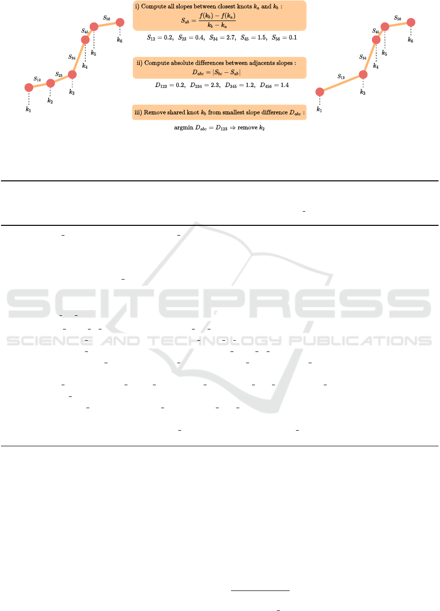
Figure 3: Example of an iteration from our proposed quantization-aware PWL Algorithm 1. The algorithm proceeds to reduce

the number of pieces by merging two similar adjacents pieces. In this ﬁgure, the slopes

and

are the most similar pieces;

therefore, the knot k

is removed.

Algorithm 1: The algorithm recursively reduced the number of pieces until the wanted number of pieces is achieved.

The algorithm needs to be provided the function to approximate

, the input scaling factor

and zero-point

, the

quantization bitwidth

and the number of linear pieces wanted. One iteration of select knots can be viewed in Figure

def select knots(knots, intercepts, pwl nb):

dknots ← knots[1:] − knots[:−1]

dintercepts ← intercepts[1:] − intercepts[:−1]

slopes ← dintercepts/dknots

if len (slopes) == pwl nb:

return knots, slopes, intercepts

else:

diff adj slopes ←



slopes[:−1]− slopes[1:]



knot index to remove ← argmin diff adj slopes

remaining knots ← knots.remove(knot index to remove)

remaining intercepts ← intercepts.remove(knot index to remove)

return select knots(remaining knots, remaining intercepts, pwl nb)

def create quantization aware pwl(f, input scale, input zero point, b, pwl nb):

quantized knots ← [0,...,2

− 1] // Generate every q

knots ← input scale  (quantized knots − input zero point) // Generate every r

intercepts ← f (knots)

{knots, slopes, intercepts} ← select knots(knots, intercepts, pwl nb)

return knots, slopes, intercepts

units. The decoder consists of 3 LSTM layers of units

1024 with Bahdanau attention on the encoder’s hidden

states and residual connections between each layer.

The dataset preprocessing is exactly the same as in

Wang et al. (2019b). We train the model for 30 epochs

on one V100 GPU, which takes approximately 6 days

to complete. We use a batch size of 24 while limiting

the maximum number of tokens in a mini-batch to

26000. Adam is used with a starting learning rate of

0.001

, which is divided by 2 when the validation set

metric plateaus without a relative decrease of

−4

in performance. Cross-entropy with uniform label

smoothing

α = 0.1

(Szegedy et al., 2016) is used as

a loss function. At evaluation time, the model predic-

tions are weighted using a pre-trained full-precision

4-layer LSTM language model (shallow fusion). Note

that we consider this language model an external com-

ponent to the ESPRESSO LSTM; we do not quantize

it due to the lack of resources. However, we already

show in our language modeling experiments that quan-

tized language models retain their performance. We

refer the reader to Wang et al. (2019b) and training

script

for a complete description of the experimental

setup. We initialize the quantized model from the pre-

trained full-precision ESPRESSO LSTM. We train the

https://github.com/freewym/espresso/blob/master/

examples/asr librispeech/run.sh

ICPRAM 2022 - 11th International Conference on Pattern Recognition Applications and Methods

120

quantized model for only 4 epochs due to the lack of

resources. The quantized model is trained on 6 V100

GPUs where each epoch takes 2 days, so a total of

48 GPU days. The batch size is set to 8 mini-batch

per GPU with maximum 8600 tokens. We made these

changes because otherwise, the GPU would run out of

VRAM due to the added fake quantization operations.

For the ﬁrst half of the ﬁrst epoch, we gather statistics

for quantization parameters then we enable QAT. The

activation functions are swapped with quantization-

aware PWL in the last epoch. The number of pieces

for the quantization-aware PWLs is 96, except for the

exponential function in the attention, which is 160 as

we found out it was necessary to have more pieces

because of its curvature. The number of pieces used

is higher than in the language modeling experiments

we did. However, the difference is that the inputs to

the activation functions are 16-bit rather than 8-bit al-

though the outputs are still quantized to 8-bit. It means

we need more pieces to capture the inputs resolution

better. Note that it would not be feasible to use a 16-bit

Look-Up Table to compute the activation functions due

to the size and cache misses, whereas using 96 pieces

allows for a 170x reduction in memory consumption

compared to LUT.

iRNN: Integer-only Recurrent Neural Network

121