
Understanding Summaries: Modelling Evaluation in Extractive
Summarisation Techniques
Victor Margallo
a
PublicSonar, Zuid Hollandlaan 7, The Hague, The Netherlands
Keywords:
NLP, Extractive Summarisation, Evaluation, Summary Quality Modelling.
Abstract:
In the task of providing extracted summaries, the assessment of quality evaluation has been traditionally tack-
led with n-gram, word sequences, and word pairs overlapping metrics with human annotated summaries for
theoretical benchmarking. This approach does not provide an end solution for extractive summarising algo-
rithms as output summaries are not evaluated for new texts. Our solution proposes the expansion of a graph
extraction method together with an understanding layer before delivering the final summary. With this tech-
nique we strive to achieve a categorisation of acceptable output summaries. Our understanding layer judges
correct summaries with 91% accuracy and is in line with experts’ labelling providing a strong inter-rater reli-
ability (0.73 Kappa statistic).
1 INTRODUCTION
One of the multiple applications of Natural Language
Processing is summarisation. The goal of such a task
is to extract or generate a shorter version of the origi-
nal text. There are two approaches for summarisation;
the first one is extractive and the second one is gener-
ative.
Extractive summarisation makes use of literal sen-
tences or keywords from the original text ranking
them with an importance metric. On the other hand,
generative models rely predominantly on Deep Learn-
ing techniques that decode the original text into a
shorter version, mimicking human summaries shown
in the training phase. Even though the latter strikes
to yield a more human-like synthesis, extractive sum-
marisation is unsupervised and the only technique ap-
plicable when dealing with no training datasets. Due
to the lack of availability in summarisation datasets
for minor languages, extractive methods are still of
great relevance and the main driver for this research
in the Dutch language.
Methods to address evaluation of summarising
output are limited to overlapping metrics based on n-
gram, word sequences, and word pairs ratios. These
metrics described in methods as ROUGE (Lin, 2004)
present drawbacks such as the ambiguity of the
ground truth depending on the annotators and the lack
a
https://orcid.org/0000-0002-5765-6671
of evaluation on newly summarised text. Even though
evaluation on new text is not a concerning issue in
theoretical research of the model—as it is evaluated
against a predefined ground truth—it becomes criti-
cal in a real world usage of the algorithm since it is
to be executed on new text with no manual annota-
tion for its quality evaluation. More recent research,
as in Wu et al. (2020), includes advanced text embed-
ding comparisons in order to provide a score, also in
new summaries. Yet, it is not defining a line regard-
ing quality acceptability. Hence, a gap between the
research usage and the practical usage of summaris-
ing algorithms exists. As a result of a missing qual-
ity check, extractive algorithms can deliver unsuitable
summaries for human end-readers, drawing the pur-
pose of a summarising technique—this is, shortening
input text into an output text that is concise, readable
and understandable—away.
We propose an integration of a graph model to-
gether with a layer replicating the understanding crite-
ria for a readable and correct summary. This pipeline
provides the summary, firstly created by the graph
model, as long as the understanding layer confirms
it is readable. We achieve 91% accuracy in this task.
Plus, the results show the algorithm to be in consistent
agreement with the variability of the human assess-
ment concerning summary output quality, measured
with an inter-rater reliability Kappa value of 0.73.
The paper follows with Section 2 introducing re-
lated work in the field, focusing on the nature of ex-
Margallo, V.
Understanding Summaries: Modelling Evaluation in Extractive Summarisation Techniques.
DOI: 10.5220/0010954300003116
In Proceedings of the 14th International Conference on Agents and Artificial Intelligence (ICAART 2022) - Volume 2, pages 605-611
ISBN: 978-989-758-547-0; ISSN: 2184-433X
Copyright
c
2022 by SCITEPRESS – Science and Technology Publications, Lda. All rights reserved
605

tractive summarising algorithms and the main model
evaluation method ROUGE; Section 3 describes the
data used in this research together with the criteria
established for the definition of a good quality sum-
mary, the algorithmic architecture for the solution—
from the graph model to the developed understanding
layer and its optimization—and the construction of in-
put features from source text and output text that feed
the understanding layer; finally, Section 4 and Sec-
tion 5 show the results of the research and end it with
a conclusion and future work.
2 RELATED WORK
Extractive summarisation sets its foundations on
graph-based ranking algorithms such as PageRank
(Brin and Page, 1998) and HITS (Kleinberg, 1999).
These algorithms were successfully applied to cita-
tion analysis, link-network of webpages and social
networks. The translation of these approaches to nat-
ural language tasks rendered algorithms as TextRank
(Mihalcea and Tarau, 2004) and progressive refine-
ments as in Barrios et al. (2016).
Graph-based methods utilize the holistic knowl-
edge of the text of interest in order to make local rank-
ing of sentences or words. With a structured ranking
of sentences the algorithm selects a reduced version
of the original text containing a presupposed high rel-
evancy.
The TextRank method uses the importance of ver-
tex connections to create a final score. To formalize,
given that G = (N, E) is a directed graph with nodes
N and edges E. Edges are connections between nodes
and thus, a NxN subset. For a N
i
node, TextRank sets
In(N
i
) as predecessor nodes pointing at the current N
i
node and Out(N
i
) as the nodes it points out to. The
score of N
i
is defined as:
S(N
i
) = (1 −d) +d ∗
∑
j∈In(N
i
)
1
Out(N
j
)
S(N
j
) (1)
Where d represents a damping factor to account
for the random surfer model probability Brin and
Page (1998). However, sentence units in natural text
relate to each other with similarity scores. TextRank
reshapes (1) so that a W factor captures it:
W S(N
i
) = (1−d)+d ∗
∑
W
j
∈In(N
i
)
w
ji
∑
N
k
∈Out(N
j
)
w
jk
W S(N
j
)
(2)
The score of sentences and therefore the weights
of the edges between sentences is given by the overlap
described as:
Similarity(S
i
,S
j
) =
{w
k
|w
k
∈ S
i
&w
k
∈ S
j
}
log(
|
S
i
|
) + log(|S
j
|)
(3)
Where S
i
and S
j
are composed of tokens S
i
=
w
i
1
,w
i
2
,...,w
i
N
i
that represent processed words. The re-
sulting most significant sentences—those with high-
est ranks—form the final summary representation.
In the succession of research in this field, most ef-
fort was focused on improving a key component of the
algorithm—the similarity score. Barrios et al. (2016)
show how the use of cosine distance with TF-IDF and
BM25 improve the quality of the results. Yet, one
of the drawbacks of TextRank algorithms is their dis-
ability to address the suitability of incoming natural
text. Consequently, it always produces an output re-
gardless of what input text is given. This results into
poor quality and low readability summaries for some
texts as it is illustrated in Figure 1.
Concerning the evaluation of the output, Mihal-
cea and Tarau (2004) appraise their method using the
ROUGE technique. Lin (2004) presents ROUGE as a
solution to the expensive and difficult process of hu-
man judgement on evaluating the different factors of
a resulting summary. ROUGE employs a set of refer-
ence summaries extracted by humans. The algorith-
mic solutions are then compared to the human ones
by means of co-occurrence statistics. The problem
with this approach is that we assume the reference
summary as the ground truth. However, there may
be several combinations which provide a good quality
summary that still do not match the human’s approach
(Mani, 2001). Therefore, even though ROUGE-like
metrics deliver a reliable benchmarking for fair com-
parison, with this paper we expand the evaluation
method by answering the question Can we detect a
human acceptable summary output?
We observe that, when applying these TextRank-
based algorithms, it is uncertain whether results are
summaries of good or bad quality. Given an origi-
nal text being noisy and not formally structured, the
resulted summary will be of the expected same low
quality. Likewise, if the original text does not contain
clear sentences that help summarize the content, the
output will not make sense to the reader. We can think
of an interview article formatted in dialogues. Ex-
tractive algorithms are limited to selecting sentences
and, in scenarios such as a dialogue/interview, there
are no good candidates to form a complete summary.
Another example is financial news which touch upon
many topics. Last example refers to sports articles;
we may face a long article describing all the matches
of the day. The output will not be satisfactory on sum-
marising well all the content information. Some ex-
amples of the above mentioned situations are listed in
Figure 1.
Thus, in this paper, we aim at the definition of
quality and readability for summaries delivered by
ICAART 2022 - 14th International Conference on Agents and Artificial Intelligence
606
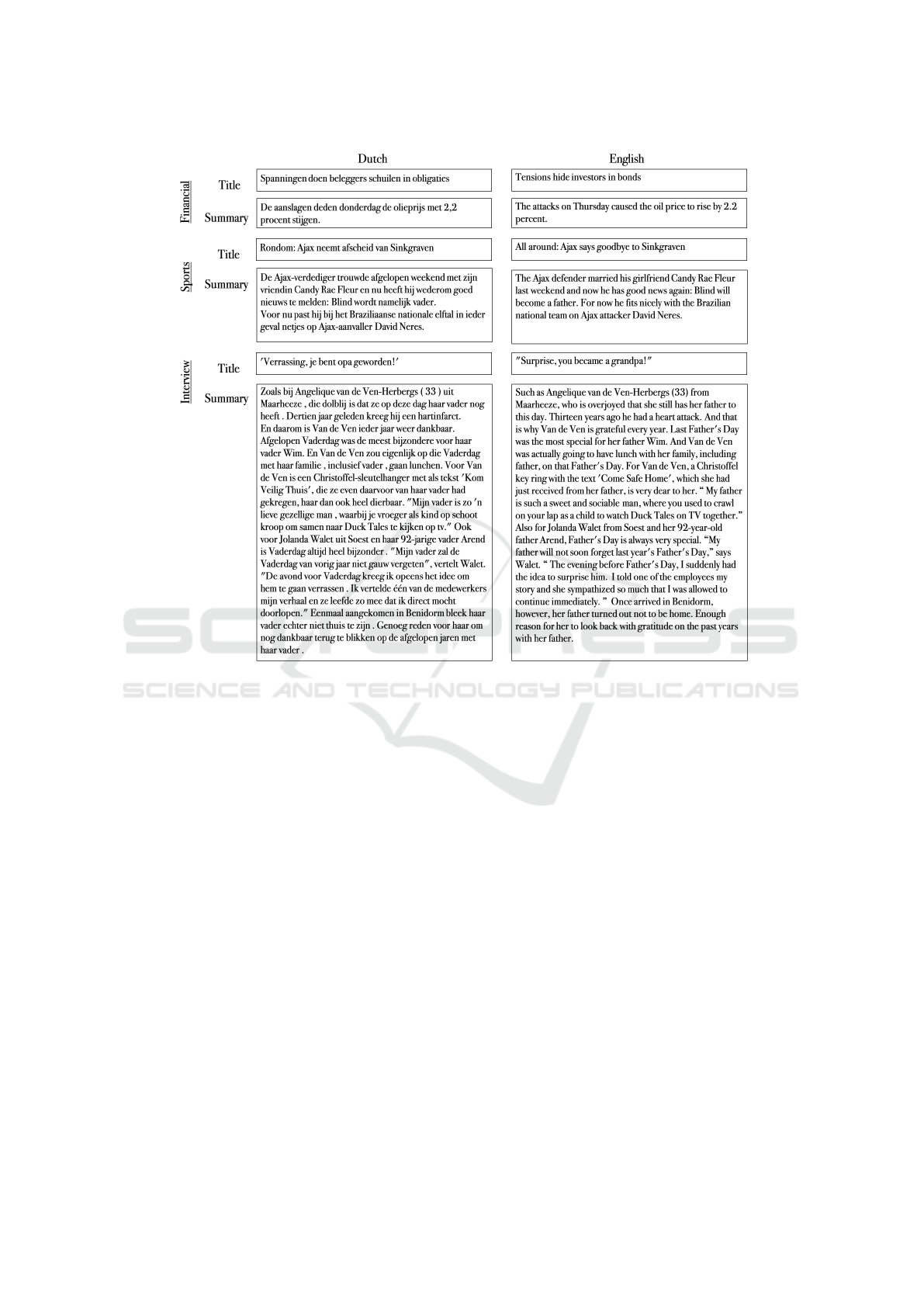
Figure 1: Examples of bad quality summaries.
TextRank methods and hereby propose an under-
standing layer to avoid poor output and solve its non-
discriminant nature.
3 METHOD
Hereinafter, we proceed to describe our modelling
methodology. The following subsections will consist
on the annotated data utilized to model decision mak-
ing on the summary output; the algorithmic architec-
ture of our solution; and the construction of input fea-
tures from both incoming and outcoming text.
3.1 Data
Our dataset is composed of 500 Dutch annotated doc-
uments forming our ground truth. The articles con-
tained in our sample have been randomly selected in
a pool of different news sources with a diverse range
of topics.
A group of experts annotated the sample dataset
following guidelines in pursuit of a harmonious an-
notation result. The annotation guidelines converge
the assessment of the summary quality in the pillars
of readability, information or content, and coherence.
Readability refers to the lack of textual barriers
or noise—for instance, misplacement or presence of
unsought characters or wrong parsing. Information
or content introduce the rules in which a summary is
considered correct when it delivers a general under-
standing of the main topic of the article. Finally, co-
herence covers the complete sense of the text. Hence,
it implies the holistic correctness of the summary—
this includes the absence of unrelated or incongruous
sentences in the summary.
Additionally, we implement an anonymous feed-
back mechanism so that reviewers can vote on the
summary independently. A majority vote decides the
final label for the summary. Herewith we hope to al-
leviate annotators’ bias in the assessment of the sum-
mary. One potential bias is, for instance, the familiar-
ity of the annotator with the topic of the text and thus,
his better understanding of a small context compared
to an uninformed annotator. Despite these efforts, it
is safe to assume discrepancies in human judgement
Understanding Summaries: Modelling Evaluation in Extractive Summarisation Techniques
607

towards the quality of the summary and therefore, we
include the Kappa statistic (Cohen, 1960; McHugh,
2012) to consider the inter-rater degree of agreement.
The Kappa statistic calculates the agreement between
two sets of annotations or evaluations considering the
possibility of random agreement.
3.2 Algorithmic Architecture
Our graph extraction pipeline is based on the algo-
rithm of Barrios et al. (2016) and works on the sen-
tence level of the text. We optimize the preprocess-
ing pipeline for the Dutch language, specifically, the
stopwords list curation, the sentence splitter and the
stemmer. The graph extraction model ranks processed
sentences on their centrality values:
centrality(S
1
,S
2
) =
n
∑
i=1
IDF(q
i
) ·
f (q
i
,S
1
) · 2.2
f (q
i
,S
1
) + 1.2 ·
1 − 0.75 + 0.75 ·
|S
1
|
avgsl
(4)
Equation 4 shows the calculation of centrality for
S
1
and S
2
which represent a pair of sentences in the
text. The variable q
i
are the terms of S
2
. IDF(q
i
) is the
function computing the Inverse Document Frequency
(Jones, 1972) of the term q
i
. In order to avoid non-
valid IDF values for terms out of the vocabulary, the
function has a floor given by 0.25 · avgIDF for those
cases. The function f (q
i
,S
1
) is the term frequency of
q
i
in S
1
. The length of S
1
in words is |S
1
| and avgsl is
the average sentence length in the original document.
The most central sentences, ordered by appear-
ance on the original article, compose the summary.
The number of sentences will be parametrized as a
preset percentage of the original length. In our re-
search, the ratio of summary sentences to original sen-
tences is set at 0.15.
Our understanding layer forms the second part of
the algorithm. This layer mimics a quality evalua-
tor in order to exclusively pass through readable and
comprehensible text. Three different models define
the architecture of this layer. An ensemble of Ran-
dom Forest, Support Vector Machine and a Neural
Network. The reason to use an ensemble of models
is to exploit the strengths of each individual compo-
nent. The strategy of bringing different classifiers to-
gether provides an improvement on the generalization
performance (G
¨
unes¸ et al., 2017). Plus, the combina-
tions of outputs reduces the probability of choosing
a poor classifier and the average error rate. Namely,
following Wolpert (1992), assuming a constant error
rate ε and the independence of classifiers, the error
rate of the ensemble benefits from the diversification
effect shown by:
e
ensemble
=
N
∑
n
N
n
ε
n
(1 − ε)
N−n
(5)
Where N is the number of classifiers in the ensem-
ble model and n is the majority voting number. The
term ε is the error rate. One of the requirements in the
selection of the components is the diversity between
them. This diversity in the classifiers will reinforce
the independence assumption of the error rate made
beforehand by a lower correlation in the predictions.
Random Forests are excellent stand-alone algo-
rithms as they are composed by an ensemble of de-
cision trees. This method bootstraps random samples
and selects a random number of features. As a result,
Random Forest becomes a robust classifier to outliers
and noise, with a good generalization to new data and
highly parallelizable (Breiman, 2001).
Support Vector Machines, on the other hand, are
suited methods for binary classification that work em-
pirically better on sparse data such as text classifica-
tion problems (Hearst et al., 1998). Its nature resides
on the distance of support vectors in order to draw a
decision boundary.
Finally, Neural Networks are connected layers
that tend to outperform Machine Learning models as
the training dataset increases. Additionally, the inclu-
sion of a sequential model allows to capture the text
linearity that Bag of Words techniques in ML mod-
els fail to address (Schuster and Paliwal, 1997; Zhou
et al., 2016).
In this paper we design a weighted voting ensem-
ble model architecture. The three models previously
mentioned are combined with different input features
explained in the next section. The ensemble model is
exposed to a Monte Carlo simulation selecting train-
ing and validation data. The process is performed
thousand times to assure the covering of most train-
ing/validation splits and help minimize the bias of
the estimates following Zhang (1993). The probabil-
ity results of the ensemble model are eventually opti-
mized by:
max(AUC) = max
Z
1
x=0
TPR
i
(FPR
−1
i
(x))dx
(6)
Where TPR is the True Positive Rate and FPR is the
False Positive Rate for every i weight distribution of
the ensemble models. Formally, we define both rates
as:
TPR
i
(T) =
Z
∞
T
f
i
1
(x
i
)dx, FPR
i
(T) =
Z
∞
T
f
i
0
(x
i
)dx
(7)
Where T is the probability threshold to classify the
prediction X and under the conditions defined by:
f
i
1
(x
i
) =
X
j
| X
j
> T
, f
i
0
(x
i
) =
X
j
| X
j
< T
(8)
The probability density function is f
1
(x) for positive
predictions and f
0
(x) for the negative ones. We define
X
j
as:
ICAART 2022 - 14th International Conference on Agents and Artificial Intelligence
608

X
j
= (w
SVM
p
j
SVM
+ w
RF
p
j
RF
+ w
NN
p
j
NN
) (9)
Where j is the different data points in the valida-
tion set and (w
SVM
,w
RF
,w
NN
) belong to a set W contain-
ing all combinatory possibilities for the weight distri-
bution of the ensemble model.
The AUC or Area Under the Curve shows the per-
formance by comparing the TPR versus FPR trade-
off. In an intuitive way, the result of AUC is the
probability of a random positive data point ranking
higher than a negative one. Section 4 will visualize
the optimal AUC in the Receiver Operating Charac-
teristic curve or ROC curve (Bradley, 1997). ROC
is the graphical representation of the AUC trade-off,
plotting the TPR against the FPR levels.
3.3 Input Features
Our input features are built in order to provide the
differentiable aspects of the text so that the ensemble
model can determine the correct class.
There are three pillars—the formatting, the se-
mantics and the syntax. The formatting of the text in-
cludes the length of the text measured on the number
sentences, the average sentence length in characters,
average number of words per sentence, and number
of dialogue dashes, colons, quotes, question and ex-
clamation marks. These features are specially deter-
minant on texts containing complex formats on which
the summarisation algorithm fails and, consequently,
translates to a non-readable summary. The semantic
layer helps define how likely a text is to be correct
or incorrect given its thematic. For instance, sports
and interview articles are prone to produce unsatis-
factory summaries. The syntax layer considers what
an acceptable concatenation of syntactic units is. This
helps detect when sentences are wrongly extracted—
we may think of two sentences put together due to a
mistake in the sentence splitter in the pre-processing.
As a result of its sequential nature, this input is only
available to the LSTM layers of the Neural Network
model.
Following Figure 2, we store the extracted for-
matting features in a Coordinate list (COO) with (row,
column, value) structure, this will help coordinate the
stacking with the semantic layer extracted through
TF-IDF (Jones, 1972) stored in Compressed sparse
row (CSR). Furthermore, we parameterize the weight
of each array before concatenating. This is defined
by α in the formatting array and β in the semantic ar-
ray. In the background α and β are subdivided into
two more parameters (ε
v
,θ
v
) for v = α,β that provide
the weight distribution to arrays from the original text
and arrays from the summarized text. This sparse ar-
ray is fed to the Random Forest and to the Support
Figure 2: Input features.
Vector Machine as well as to the dense layer of the
Neural Network. Syntax is captured by a fixed length
sequence containing the Part of Speech tags from only
the summary text. This feature is read left-to-right
and right-to-left by a Bidirectional LSTM (Bi-LSTM)
(Schuster and Paliwal, 1997).
4 RESULTS
Input weights α and β are fine-tuned on cross-
validation with grid search during warm-up simula-
tions. The ensemble model weight distribution is as-
signed to the predicted probabilities from each of the
models and optimized based on equation (6). Figure 3
shows the result of such optimization, where the best
performing weight distribution is marked with red and
visualises the True Positive Rate trade-off with the
False Positive Rate of the ensemble for the different
threshold T as explained in (7). The blue channel
in Figure 3 represents all other weight combinations
arisen from the simulations. Lastly, the grey area is
the baseline for a random guess.
Table 1 exhibits the evaluation metrics for the op-
timized understanding layer at T = 0.5. Our ensem-
ble model obtains a conclusive 90.84% accuracy on
our validation rounds. The ensemble model seems
to weaken in recalling bad quality summaries, such
lower recall determines consequently the impact on
the precision metric of good quality summaries due
to its binary outcome. This flaw in bad quality sum-
maries recall can be explained by the smaller amount
of such examples in the training phase. Overall, the
results in Table 1 show that it is possible to transmit
quality checks through an engineered formatting layer
together with the syntax and the semantics. These
findings satisfy our objective to create an algorith-
mic solution that could substitute or emulate expen-
sive manual evaluation.
Understanding Summaries: Modelling Evaluation in Extractive Summarisation Techniques
609
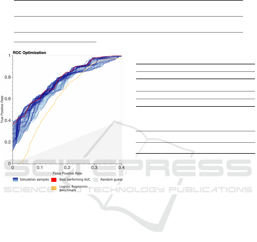
Table 1: Understanding layer: Evaluation metrics.
Label
Precision (Std.)
%
Recall (Std.)
%
F1 (Std.)
%
Samples support
Support pct.
%
Bad quality 98.65 (2.70) 64.63 (7.60) 78.09 (5.80) 3158 25.26
Good quality 89.29 (2.72) 99.70 (0.64) 94.21 (1.56) 9342 74.73
Accuracy (Std.) % 90.84 (2.33)
Figure 3: Optimization for model distribution.
Nevertheless, and despite the usefulness of the
previous metrics for reference and model fine-tuning,
we face an evaluation with different outcomes based
on the specific individuals assessing the quality of the
final summary. This lack of agreement produces po-
tential mismatches on the same summary outcome.
Thus, it is crucial to quantify the consensus between
the labelling experts and the algorithmic solution to
judge the performance of our understanding layer in
perspective. Therefore, we proceed to evaluate the
variability in the data labeled by the experts.
We introduce Cohen’s Kappa statistic (κ) (Cohen,
1960) to measure the degree of agreement or disagree-
ment happening by chance. It ranges from -1 to 1
where 0 is random chance and 1 represents perfect
agreement.
In our experiment, we merge our experts’ labels
and we include the algorithm as a second rater in or-
der to model the raters’ agreement probabilities. In
Table 2 the results for our model are listed. Table 2
are the agreement probabilities calculated from our
dataset and from the model’s results. The latter proba-
Table 2: Results of Kappa statistic through agreement prob-
abilities.
Agreement probabilities
p
o
P
max
p
Good
p
Bad
p
e
Values (%) 90.84 91.29 62.37 4.18 66.55
(a) Agreement probabilities from our testing dataset.
Kappa statistics κ κ
max
SE
κ
CI (95%)
Values 0.7262 0.7395 0.0077 [0.7185,0.7339]
(b) Kappa statistics calculated from the agreement proba-
bilities.
Table 3: Kappa agreement levels.
Std. range <0 <0.2 <0.4 <0.6 <0.8 <1
Norm. range <0 <0.15 <0.3 <0.44 <0.59 <0.74
Agreement
magnitude
None Slight Fair Moderate Substantial Almost
perfect
Note: Magnitude assessment following Landis and Koch
(1977).
bilities are the input for the calculus of the Kappa val-
ues in Table 2b. In Table 3 we provide the standard
range for equally distributed categories and the nor-
malised range for our specific sample. The standard
range is used as a Kappa benchmark established by
Landis and Koch (1977) in order to express the agree-
ment magnitude for different Kappa values. The nor-
malised range takes into account the unbalanced dis-
tribution of our classes and scales the standard range
based on the maximum Kappa value. Our understand-
ing layer achieves a 0.7262 Kappa statistic of a maxi-
mum of 0.7395. By considering chance agreement in
an ambiguous qualitative task such as summary eval-
uation, the finding of a strong Kappa (0.7262) shows a
behaviour almost completely in line with the expected
behaviour from a human data labeler.
5 CONCLUSION AND FUTURE
WORK
In the lack of quality assessment of extractive sum-
maries, we present an understanding layer in order to
determine the readability of the outcome. We have
shown how we may translate human assessment of
summaries output into a modelling process that suc-
ICAART 2022 - 14th International Conference on Agents and Artificial Intelligence
610

cessfully performs the task with 91% accuracy. Fur-
thermore, our Kappa statistic (0.73) reinforces a con-
sistent agreement between algorithm’s and expert’s
summary labelling. This solution links the evalua-
tion of co-reference solutions for benchmarking (Lin,
2004) to an applicable solution for real summary un-
derstanding.
Future research will focus on the readability of the
models. This refers to whether we may have a snap-
shot from the ensemble model of the main features
delivering the final decision. In other words, we want
to be knowledgeable of the relevance of the format-
ting, semantic and syntactic layers on the result. This
would elucidate the understanding of the potential for
new applications regarding the machine-human cor-
relation on decision making in the task of summary
evaluation.
Lastly, the scope of this study is limited to the
Dutch language. It is to be expected a similar perfor-
mance in close relative languages such as German and
English, yet challenges increase in more distant types.
Therefore, modelling techniques should be fine-tuned
and adapted to each specific language to validate the
results previously presented.
REFERENCES
Barrios, F., Lopez, F., Argerich, L., and Wachenchauzer,
R. (2016). Variations of the similarity function
of textrank for automated summarization. CoRR,
abs/1602.03606.
Bradley, A. P. (1997). The use of the area under the
roc curve in the evaluation of machine learning algo-
rithms. Pattern recognition, 30(7):1145–1159.
Breiman, L. (2001). Random forests. Machine learning,
45(1):5–32.
Brin, S. and Page, L. (1998). The anatomy of a large-scale
hypertextual web search engine.
Cohen, J. (1960). A coefficient of agreement for nominal
scales. Educational and psychological measurement,
20(1):37–46.
G
¨
unes¸, F., Wolfinger, R., and Tan, P.-Y. (2017). Stacked
ensemble models for improved prediction accuracy. In
Proc. Static Anal. Symp, pages 1–19.
Hearst, M. A., Dumais, S. T., Osuna, E., Platt, J., and
Scholkopf, B. (1998). Support vector machines. IEEE
Intelligent Systems and their Applications, 13(4):18–
28.
Jones, K. S. (1972). A statistical interpretation of term
specificity and its application in retrieval. Journal of
documentation.
Kleinberg, J. M. (1999). Authoritative sources in a hy-
perlinked environment. Journal of the ACM (JACM),
46(5):604–632.
Landis, J. R. and Koch, G. G. (1977). The measurement of
observer agreement for categorical data. biometrics,
pages 159–174.
Lin, C.-Y. (2004). Rouge: A package for automatic evalua-
tion of summaries. Text summarization branches out,
page 74–81.
Mani, I. (2001). Automatic summarization. J. Benjamins
Pub. Co.
McHugh, M. L. (2012). Interrater reliability: the kappa
statistic. Biochemia Medica, page 276–282.
Mihalcea, R. and Tarau, P. (2004). Textrank: Bringing or-
der into text. Proceedings of the 2004 Conference on
Empirical Methods in Natural Language Processing,
page 404–411.
Schuster, M. and Paliwal, K. K. (1997). Bidirectional re-
current neural networks. IEEE transactions on Signal
Processing, 45(11):2673–2681.
Wolpert, D. H. (1992). Stacked generalization. Neural net-
works, 5(2):241–259.
Wu, H., Ma, T., Wu, L., Manyumwa, T., and Ji, S.
(2020). Unsupervised reference-free summary qual-
ity evaluation via contrastive learning. arXiv preprint
arXiv:2010.01781.
Zhang, P. (1993). Model selection via multifold cross vali-
dation. The Annals of Statistics, 21(1):299–313.
Zhou, P., Qi, Z., Zheng, S., Xu, J., Bao, H., and Xu, B.
(2016). Text classification improved by integrating
bidirectional lstm with two-dimensional max pooling.
arXiv preprint arXiv:1611.06639.
APPENDIX
In Table 2 we define p
o
as the raters’ accuracy.
The maximum agreement probability is P
max
=
∑
k
i=1
min(P
i+
,P
+i
) where P
i+
and P
+i
are the row and
column probabilities from the original raters’ matrix.
p
Good
and p
Bad
are the probability of random agree-
ment for the different summary categories. p
e
is
the random probability for both categories together,
thus, p
e
= p
Good
+ p
Bad
. Kappa value is defined as
κ =
p
o
−p
e
1−p
e
. The maximum value for the unequal
distribution of the sample is κ
max
and is calculated
by κ
max
=
P
max
−P
e
1−P
e
. The standard error and confi-
dence interval are calculated by SE
κ
=
q
p
o
(1−p
o
)
N(1−p
e
)
2
and
CI : κ ± Z
1−α/2
SE
κ
respectively.
Understanding Summaries: Modelling Evaluation in Extractive Summarisation Techniques
611
