Incremental Scheduling of the Time-triggered Trafﬁc on TTEthernet

Network

Zden

ek Hanz

alek

and Jan Dvo

CIIRC, Czech Technical University in Prague, Jugoslavskych partyzanu 1580/3, Prague, Czech Republic

Keywords:

Scheduling, Ethernet, Time-triggered.

Abstract:

Complex systems are often developed incrementally when subsequent models must be backward compatible

with the original ones. The need to exchange high-volume data, for example, multimedia streams in the avionic

systems, together with safety-critical data, puts demands on both the high bandwidth and the deterministic

behavior of the communication. TTEthernet is an Ethernet based protocol that enables the transmission of

the time-triggered messages. Thus, synthesizing a good schedule that meets all the deadline requirements and

preserves the backward compatibility with the schedules of preceding models is essential for the performance

of the whole system. In this paper, we study the problem of designing periodic communication schedules

for time-triggered trafﬁc. The aim is to maximize the uninterrupted gap for the remaining non-deadline-

constrained trafﬁc. The provided scheduling algorithm, based on MILP and CP formulation, can obtain good

schedules in a reasonable time while preserving the backward compatibility. The experimental results show

that the time demands of the algorithm grows exponentially with the number of messages to be transmitted,

but, even for industrial-sized instances with more than 2000 messages, the algorithm is able to return the close

optimal schedules in the order of hundreds of seconds.

1 INTRODUCTION

The development process in many industrial ﬁelds,

e.g., automotive or avionics, is based on incremen-

tal steps where new models are an evolution of the

previous ones. This incremental process enables the

cost-efﬁcient development for companies and reduces

the test effort. Moreover, the customer is guaran-

teed that the new model is an upgraded version of

the model that he or she is comfortable with. These

beneﬁts are a side effect of the backward compatibil-

ity that should be assured among incremental devel-

opment steps. Backward compatibility affects exter-

nal systems, e.g., human-machine interface, as well

as internal ones such as the communication subsys-

tem. The backward compatibility in communication

subsystems signiﬁcantly reduces the costs spent on

debugging, testing, and maintenance as newly devel-

oped Electronic Control Units (ECUs) and diagnos-

tic tools can follow the agreement on the sharing of

communication resources achieved in previous devel-

opment steps.

The incremental development process is already

https://orcid.org/0000-0002-8135-1296

https://orcid.org/0000-0002-7004-9358

ingrained in the industrial practice. However, there

is an ongoing effort to develop and produce new

models even more cost-efﬁciently. One possibility

on how to reduce production costs in complex inter-

connected systems is to combine safety-related com-

munication together with non-critical communication

into one common medium (Li et al., 2019). Safety-

related communication requires determinism, while

non-critical communication demands a huge band-

width without hard timing constraints. In the past,

these two communication ﬂows were conducted sep-

arately, as there were no communication protocols

that could handle the requirements of both. However,

modern protocols, like TTEthernet (commercial name

stands for Time-Triggered Ethernet), were developed

to bear such a difﬁcult task.

In TTEthernet, safety-related communication is

exchanged based on a periodic time-triggered com-

munication schedule, while non-critical communica-

tion ﬁlls the empty gaps in the schedule. Such a com-

munication schedule has to be designed in a way that

all the deadline requirements are met to enable the re-

liable and deterministic operation of the application.

The creation of the schedule involves additional com-

plexity compared to the bus or passive star topolo-

302

Hanzálek, Z. and Dvo

rák, J.

Incremental Scheduling of the Time-triggered Trafﬁc on TTEthernet Network.

DOI: 10.5220/0010953700003117

In Proceedings of the 11th International Conference on Operations Research and Enterprise Systems (ICORES 2022), pages 302-313

ISBN: 978-989-758-548-7; ISSN: 2184-4372

l,m

m,o

o,p

p,q

p,u

o,n

n,r

n,m

t,m

n,s

m,t

m,l

o,m

m,n

s,n

n,o

r,n

p,o

u,p

q,p

Figure 1: An example of the TTEthernet network topology

with the routing and scheduling of message m

from node l

to node q.

gies of networks like FlexRay (International Organi-

zation for Standardization, 2015; Dvorak and Han-

zalek, 2016) or CAN (Waszniowski et al., 2009) be-

cause TTEthernet supports complex switched topolo-

gies (Tuohy et al., 2015). These aspects, together with

the real case problem proposed by our avionics in-

dustry partner, have motivated us to face the prob-

lem of scheduling time-triggered communication on

the TTEthernet network while keeping the incremen-

tal development process in mind.

The paper presents the algorithm for creating

schedules for time-triggered trafﬁc on the TTEther-

net network while maximizing the minimal guaran-

teed continuous gap for the trafﬁc with lower critical-

ity. The study aims to develop the periodic scheduling

algorithm, which preserves the backward compatibil-

ity with the original schedule. Finally, the inﬂuence

of the backward compatibility on the communication

schedule is analyzed.

1.1 TTEthernet Overview

TTEthernet is an extension of Ethernet for determinis-

tic communication developed as a joint project among

the Vienna University of Technology (Kopetz et al.,

2005), TTTech, and Honeywell, and standardized as

SAE AS 6802 (SAE International, 2011) in 2011. It

operates at Level 2 of the ISO/OSI model, above the

physical layer of Ethernet. It requires a switched net-

work with full-duplex physical links, such as Auto-

motive Ethernet standard 1000BASE-T1. An exam-

ple of the TTEthernet topology is depicted in Fig. 1.

The global time in the system is assured by the

clock synchronization protocol, where the clocks of

all the interconnected ECUs are being synchronized

periodically. Every synchronization period is called

an integration cycle.

RC1

RC2

RC3

Integration cycles

time [ms]

Part of the integration cycle

used by TT communication

minimal

guaranteed gap

Figure 2: The example of the communication on a link in

one cluster cycle.

The trafﬁc with various time-criticality is inte-

grated into one physical network. There are three traf-

ﬁc classes in TTEthernet. These classes, ordered by

decreasing priority, are Time-Triggered (TT), Rate-

Constrained (RC) and Best-Effort (BE) trafﬁc.

The TT trafﬁc class has the highest priority. A

jitter shorter than µs can be achieved on a physical

layer (the physical layer jitter also depends on the

connected network devices). The TT messages are

periodic. We assume that they are strictly periodic

(i.e., no jitter in application level is allowed) in agree-

ment with (Tamas-Selicean et al., 2015b). The least

common multiple of their period is called the cluster

cycle.

For trafﬁc with less strict timing requirements,

the RC trafﬁc class can be used. This trafﬁc class

conforms to the ARINC 664p7 speciﬁcation (ARINC

(Aeronautical Radio, Inc.), 2009), also called AFDX.

The RC trafﬁc represents event-triggered communi-

cation, which does not follow any schedule known in

advance.

A simple example of the TT trafﬁc, together with

the RC trafﬁc on one direction of a physical link, is

presented in Fig. 2. In the ﬁgure, the particular inte-

gration cycles are situated in rows, and the horizontal

axis represents the time instants in the particular inte-

gration cycle. The length of the cluster cycle (40 ms)

is equal to four times the length of the integration cy-

cle (10 ms) here. The ﬁgure shows that messages T T

T T

and T T

have the same period (twice the duration

of the integration cycle - i.e., 20 ms) and T T

has a pe-

riod equal to four times the integration cycle length.

The dark message at the beginning of each integration

cycle is the synchronization message.

Standard Ethernet trafﬁc can be transmitted

through the network too. Such trafﬁc is called the

Best-Effort (BE) trafﬁc and has the lowest priority.

When the TT trafﬁc is used together with other

trafﬁc classes, a TT message could be delayed by an-

other RC or BE message. The delay happens when

a TT message arrives while an RC or BE message is

in transmission. The Timely block integration pol-

icy, which causes no extra delay of the TT trafﬁc, is

Incremental Scheduling of the Time-triggered Trafﬁc on TTEthernet Network

303

used in this paper. In this case, an RC or BE mes-

sage can only be transmitted if there is enough time

for the transmission of the entire message before the

next TT message is scheduled. If there is insufﬁcient

time, the transmission of the RC or BE message is

postponed until after the TT message is transmitted.

It additionally means that the TT trafﬁc follows the

schedule without any delays.

1.2 Related Works

The area of time-triggered communication schedul-

ing on Ethernet-based networks has already been ex-

amined in many publications. Steiner (Steiner, 2010)

was among the ﬁrst to study the problem. They de-

scribed the basic constraints for scheduling the com-

munication in the TTEthernet network and provided

the Satisﬁability Modulo Theories (SMT) formula-

tion that was able to ﬁnd a feasible schedule for small

instances with up to 100 messages. The concept of

schedule porosity was introduced in (Steiner, 2011).

The porosity (the allocated blank slots for RC mes-

sages spread over the integration cycle) is introduced

to the schedule to decrease the delay posed on RC

trafﬁc by TT trafﬁc. To evaluate the impact of the

porosity on the RC trafﬁc, Steiner et al. provided a

pessimistic worst-case delay calculation, which was

consequently tightened by a new method in (Tamas-

Selicean et al., 2015b). A more detailed study of

the impact of the time-triggered schedule on the RC

communication has been presented in (Boyer et al.,

2016). In (Tamas-Selicean et al., 2015a), the au-

thors employed the TabuSearch algorithm to over-

come the scalability problem of previous SMT for-

mulations. As noted by (Steiner et al., 2015), poros-

ity scheduling has a disadvantage that gaps introduced

at the beginning of the scheduling process do not

consider the proﬁle of the RC trafﬁc. The concept

of porosity is also weak in the case of scheduling

TT messages with short periods. Wang et al. (Wang

et al., 2018) used back-to-back schedule optimization,

which aims to minimize the standard deviation of the

messages offset in the integration cycle (hence, cre-

ate as compact schedule as possible), to overcome

the weakness of the porosity approach. The con-

cept of minimization of the TT communication block

length, called makespan minimization, was presented

in (Dvo

ak et al., 2017). The paper formulates the

scheduling problem as an RCPSP model to solve the

problem efﬁciently. However, the method did not al-

low one to preserve the backward compatibility, and

the quality of the resulting schedule was limited by

the use of naive shortest-path-tree routing algorithm.

Pozo et al. in (Pozo et al., 2019) used a divide-and-

conquer method to overcome the scheduling scalabil-

ity limitations in large-scale hybrid networks consid-

ered to be used in, for example, smart cities in the

future.

Based on the given TTEthernet communication

schedule, Craciunas et al. scheduled the tasks on the

communication endpoints in (Craciunas et al., 2014).

Several authors presented a holistic scheduling algo-

rithm that makes schedules of communications and

computations together (Craciunas and Oliver, 2016;

Minaeva et al., 2018).

The closely related problem to TTEthernet

scheduling is the scheduling of TT communication for

IEEE 802.1Qbv, which is the standard of the IEEE

Time-Sensitive Networking group (see discussion in

(Moutinho et al., 2019)). Craciunas et al. derived the

scheduling constraints for the TT communication on

IEEE 802.1Qbv in (Craciunas et al., 2016) and pro-

vided an SMT model that aims to minimize the num-

ber of queues needed to schedule a given set of mes-

sages. Even though the TTEthernet and 802.1Qbv

shares many features, the queues with a limited num-

ber of priorities used in 802.1Qbv introduces changes

to the problem statement (Vlk et al., 2022).

All the published papers aim to create schedules

from scratch, and none of them considers backward

compatibility with the preceding systems, which lim-

its the use of the proposed method in industries with

an incremental development process.

1.3 Paper Outline

The main contributions of this paper are:

1. The formal description of the incremental TTEth-

ernet scheduling problem with deadline con-

straints.

2. The three-stage heuristic algorithm, which in-

cludes

• the routing algorithm that balances the commu-

nication load among the links

• the message-to-integration-cycle assignment

algorithm that balances the communication

load among the integration cycles

• the message scheduling method based on the

constraint programming model of the problem

3. An examination and discussion of the impact of

the incremental aspect on TTEthernet scheduling.

4. An evaluation of the proposed algorithm from

quality and performance point of view.

The paper is organized as follows: Section 2 de-

scribes the studied problem of the incremental TT

ICORES 2022 - 11th International Conference on Operations Research and Enterprise Systems

304

message scheduling in the TTEthernet network com-

prehensively. In Section 3, the proposed method of

the schedule creation is described consisting of a mes-

sage routing method, a load-balancing heuristic, and

a CP based formulation of the scheduling problem.

The method and the impact of the backward compat-

ibility on the scheduling are evaluated and discussed

in Section 4. Section 5 concludes the paper.

2 PROBLEM STATEMENT

This paper aims to design a method for ﬁnding feasi-

ble strictly periodic schedules for time-triggered com-

munication on the TTEthernet network so that the

maximal part of the remaining bandwidth can be pre-

served for the RC and BE messages, the timing con-

straints are satisﬁed, and the backward compatibility

with the original schedule is preserved. All aspects of

the tackled problem are described in this section.

2.1 Messages

Each message m

from a set of the TT messages M

that is to be scheduled has the following parameters:

• t

- period

• c

- message length in the number of bits consist-

ing of a payload, headers and interframe gap

• d

- deadline

• r

- release date

• q

- identiﬁer of the transmitting node

• Q

- set of the receiving node identiﬁers (the set

contains only one receiving node in the case of a

unicast message)

The message period t

is assumed to be an integer

multiple of the length of the integration cycle ic. The

length of the resulting schedule is determined by the

length of the cluster cycle cc. The cluster cycle con-

sists of set of the integration cycles I. The transmis-

sion time of message m

has to be smaller than or

equal to the duration of the integration cycle (it would

not be possible to send a synchronization message

otherwise), and its length c

does not exceed the max-

imal Ethernet frame length of 1530 bytes. Deadline

and release date r

are assumed to have the value in

the range 0 ≤ r

≤ d

≤ t

2.2 Network Topology

The TTEthernet topology consists of nodes and links

which interconnect them. The nodes e

∈ E are

divided into two classes: redistribution nodes E

l,m

m,o

m,l

o,m

the same

message occurrence

the same

message instance

Figure 3: Visualization of the difference between message

occurrence and message instance.

and communication endpoints E

. The communica-

tion endpoints are nodes that generate or process the

data (e.g., sensors, actuators, control units, and other

ECUs). Thus, only the identiﬁer of a communication

endpoint can be assigned to message m

as transmitter

or one of the receivers from set Q

. The redistribu-

tion nodes, on the other side, are switches without any

of their own data to transmit and serve as intermediary

nodes for the communication. In Fig. 1, the commu-

nication endpoints are titled by ”ECU”, and the re-

distribution nodes have arrows drawn on the top side.

The front side of each node is labeled by its name.

Each hop in the network introduces a technical de-

lay caused by queuing in the ingress and egress port.

Such a delay in a switch is represented by parame-

ter τ for the TT messages. The value of τ can be in

the range from 1 µs to 2.4 µs according to the network

conﬁguration (Steinbach et al., 2010).

Each link k

i, j

from a set of links K connects two

nodes e

and e

. This connection covers just one di-

rection of the full-duplex communication. Therefore,

two links k

i, j

and k

j,i

model one full-duplex physical

link between nodes e

and e

. These two links are

two independent resources from the scheduling point

of view. The instance of message m

in link k

l,m

called a message instance m

l,m

. The set of all the

message instances is denoted by MI. All the transmis-

sions of some message m

in one particular link repre-

sent the same message instance. The message occur-

rence, on the other hand, represents all the transmis-

sions of some message m

in one particular integration

cycle. The difference between the message instance

and the message occurrence is graphically explained

in Fig. 3. The ﬁgure shows the detailed view on the

sub-segment of the network topology from Fig. 1 with

node e

, e

and e

only. Both links of any physical

link are labeled here already.

2.3 Message Routing

A sequence of the links S

= (k

l,m

m,o

,...,k

p,q

) repre-

sents the routing path of message m

from transmitter

Incremental Scheduling of the Time-triggered Trafﬁc on TTEthernet Network

305

= e

to receiver e

∈ Q

through the redistribution

nodes e

,...,e

. The union of all the routing paths

∪S

|∀q ∈ Q

for a given message m

determines the

routing tree S

. For example, the transmission of mes-

sage m

through routing path S

is presented in Fig. 1.

Only one direction of each physical link is labeled in

the ﬁgure for the sake of simplicity. The routing paths

are not known in advance. Therefore, ﬁnding the

appropriate routing trees is part of the optimization

process.

2.4 Original Schedule

Additionally, the original schedule is given for the in-

cremental scheduling. The original schedule deﬁnes

the start time of transmissions for the message in-

stances ˜m

k,l

from the subset of the message instances

MI ⊂ MI which are already present in the original

schedule. The original schedule can be determined

for a subset of messages as well as for a subset of its

message instances. This representation of the origi-

nal schedule even allows the extension of the topol-

ogy as well as the extension of the set of receivers for

the already present messages. More precisely, all the

modiﬁcations of the topology and message set that do

not force the backward compatibility to be broken are

allowed in the incremental development process.

2.5 Schedule

The schedule is so-called strictly periodic, which

means that the next message occurrence of message

in a particular link appears in the schedule exactly

time units after the current one. Therefore, the po-

sitions of all the message occurrences of message m

in the strictly periodic schedule can be deduced from

the position of the ﬁrst message occurrence and its

periodicity.

A feasible schedule has to fulﬁll the following

hard constraints:

Completeness Constraint: Each message m

∈ M

has to be scheduled.

Contention-free Constraint: Any link is capable of

transferring at most one message at a time.

Timing Constraint: Each message has to be trans-

mitted after its release date and received by all the

receivers before its deadline.

Transmission Compactness Constraint: The mes-

sage transition from transmitting node q

to all the

receivers from Q

has to be accomplished in one in-

tegration cycle.

Backward Compatibility Constraint: The start of

transmission time must be preserved for all the mes-

sage instances participating in the original schedule.

Precedence Constraint: Message m

has to be sched-

uled in link k

m,o

at least τ time units after it is sched-

uled in k

l,m

if k

l,m

precedes k

m,o

in S

2.6 Objective

The coherent TT trafﬁc segment should be com-

pressed as much as possible to preserve the maxi-

mum part of the remaining bandwidth for the RC and

BE trafﬁc. This idea follows the practice from the

FlexRay bus or Proﬁnet, where the dedicated commu-

nication segment is allocated for the TT trafﬁc. The

TT trafﬁc can be scheduled at the beginning of the in-

tegration cycle, and the remaining coherent gap in the

integration cycle without the TT trafﬁc is preserved

for the RC and BE trafﬁc. The gap, which is the short-

est among all the links, is denoted as a minimal guar-

anteed gap (see Fig. 2). Considering the constraints

and aspects above, the goal of the scheduling is to ﬁnd

a feasible schedule for the TT messages, which max-

imizes the minimal guaranteed gap.

3 ALGORITHM

The described problem is extensively complex as

it involves scheduling together with routing. The

algorithm that would solve the whole problem at

once would put extreme demands on the computa-

tional resources or time needed to ﬁnd the solution.

Thus, the incremental scheduling problem proposed

in the paper is decomposed into three subproblems

to tackle the computational effort. The solution of

each subproblem ﬁxes some decisions for the sub-

sequent problem. Hence, the incremental schedul-

ing algorithm can be considered as being divided into

three stages. In the ﬁrst stage (Sec. 3.1), the routing

of the messages is established. In the second stage

(Sec. 3.2), the algorithm ﬁnds the assignment of the

messages to the particular integration cycles. The

transmission times for each message in each link are

decided in the last stage (Sec. 3.3).

3.1 Messages Routing Problem

The network topology is often a tree in industrial net-

works. It means that there are no cycles and, there-

fore, only one possible path from a communication

endpoint to any other endpoint exists. Thus, the deter-

mination of the routing is trivial in such a case. How-

ever, the TTEthernet does not restrict the network

topology to the tree. The cycles introduce new redun-

dant paths for messages that can serve as a backup

during a partial network malfunction. Moreover, the

ICORES 2022 - 11th International Conference on Operations Research and Enterprise Systems

306

appropriate selection of the routing path of the mes-

sage can balance the load among the network. Thus,

redundant paths can remove the bottleneck of the tree

topology. However, the TT messages have to know

which path they are routed through in advance.

min F

s.t. f

l,m

≤ F ∀k

l,m

∈ K

∑

l,m

· x

i,l,m

= f

l,m

∀k

l,m

∈ K

∑

i,l,m

= 1 ∀m

∈ M; ∀m ∈ Q

∑

i,l,m

≥ 1 ∀m

∈ M; l = q

∑

i,l,m

≤

∑

i,m,k

∀m

∈ M; ∀m ∈ E

∑

i,l,m

≤ 1 ∀m

∈ M; ∀m ∈ E

∑

i,l,m

≥

∑

i,m,k

deg

−

(m)

∀m

∈ M; ∀m ∈ E

i,m

≥ 1 + s

i,l

− B + Bx

i,l,m

∀m

∈ M; ∀k

l,m

∈ K

i,m

≤ 1 + s

i,l

+ B − Bx

i,l,m

∀m

∈ M; ∀k

l,m

∈ K

i,l

= 0 ∀m

∈ M; l = q

i,l,m

= 1 ∀m

l,m

∈

i,l,m

∈ {0,1} ∀m

∈ M; ∀l,m ∈ E

l,m

∈ Z

∀l, m ∈ E

F ∈ R

i,l

∈ Z

∀m

∈ M; ∀l ∈ E

(1)

Therefore, the ﬁrst stage of the algorithm ﬁnds the

routing. In accordance with the claim above, the al-

gorithm aims to ﬁnd such a routing that the network

load is as balanced among the links as possible. The

balanced network gives a good premise that the result-

ing communication schedules will be shorter than in

the case of an unbalanced network. Thus, this routing

objective corresponds to the aims of the scheduling

algorithm.

An MILP model is used to solve the routing sub-

problem and decide routing tree S

for each message.

The binary variable x

i,l,m

decides whether the mes-

sage m

is routed through the link k

l,m

, and variable

i,m

represents the load of the link k

l,m

. The real vari-

able F is, consequently, the load of the busiest link.

The auxiliary variable s

i,l

assigns a numerical label to

each node e

for each message m

. The label deter-

mines the depth of the node e

in the routing tree S

The artiﬁcial constant B represents any number that is

bigger than the maximal depth (max s

i,l

). Parameter

l,m

represents the transmission time of message m

link l

l,m

. Note, that if the links are conﬁgured to have

a different bandwidth, then the transmission time of

the same message varies among the links.

The objective of the MILP model minimizes the

load of the busiest link. The ﬁrst constraint, together

with the objective, ensures that the value of F equals

the load of the busiest link. The second constraint cal-

culats the load f

l,m

for each link. The third and fourth

constraints force the routing path for each message to

also contain the receiving nodes and the transmitting

node. The ﬁfth, sixth, and seventh constraint assure

that the redistribution nodes serve as the inner nodes

of the routing tree. The eighth, ninth and tenth con-

straints guarantee the routing tree of any message not

to contain the cycle. B represents any constant that is

larger than the number of nodes in the topology here.

Its aim is to make the model ignore the constraints

if the value of x

i,l,m

is equal to zero. The eleventh

constraint forces the resulting routing to satisfy the

backward compatibility.

The routing tree S

deﬁnes the set of links in which

the message is to be scheduled and speciﬁes the prece-

dence relations among the message instances.

3.2 Integration Cycle Assignment

Problem

To distribute the messages among the integration

cycles, we used an idea from the multiprocessor

scheduling area. In the area, if all the workload of the

tasks is distributed among the processors evenly, then

the part of the integration cycle used by the TT com-

munication has a good chance to be minimal. Follow-

ing that, the algorithm tries to distribute the messages

among the integration cycles evenly. All the prece-

dence constraints, the time lags imposed by the switch

delay τ, and the deadline constraints are relaxed here.

The integration cycle assignment problem is formu-

lated as the following MILP model 2.

The binary variable a

i, j

= 1 iff message m

is as-

signed to the integration cycle j ∈ {0 ...t

}. Simi-

larly, the binary parameter ˜a

i, j

= 1 iff message m

was scheduled to the integration cycle j ∈ {0 ...t

}

in the original schedule. The ﬁrst constraint assures

that the ﬁrst message occurrence appears in exactly

one of the possible integration cycles. Thus, it sat-

isﬁes the completeness constraint. The second con-

straint makes the variable z have the value equal to

or greater than the time needed to exchange all the

messages in any integration cycle of any link in the

network. The constraint is evaluated for each link and

each integration cycle in the cluster cycle so that the

transmission times of all the message occurrences as-

signed to the particular integration cycle in the given

link are summed up. The resulting total time must be

less than or equal to variable z. The aim of the MILP

Incremental Scheduling of the Time-triggered Trafﬁc on TTEthernet Network

307

model is to ﬁnd such an assignment that minimizes

z. Thus, the maximal time needed for the message

exchange among all the resources is minimized. The

third and fourth constraint force the messages to be

assigned to the integration cycle, which can satisfy the

release date and deadline constraints. The last con-

straint forces the messages from the original schedule

to be assigned to the corresponding integration cycle

in the new schedule.

min

i, j

s.t.

∑

i, j

= 1 ∀i ∈ M

∑

∈k

l,m

· a

i, j mod t

≤ z ∀ j,l,m | j ∈ {0...

}

i, j

= 0 ∀i, j | d

< j · ic

i, j

= 0 ∀i, j | r

> (j + 1) · ic

i, j

= 1 ∀i, j | ˜a

i, j

= 1

i, j

∈ {0,1}; z ∈ R ∀i, j

(2)

The resulting assignment balances the load among the

integration cycles, follows the routing of the mes-

sages, and preserves the timing and backward com-

patibility constraints.

3.3 Link Schedules Creation Problem

The constraint programming model is employed to

create the resulting schedule. For the description of

the model, the IBM CP Optimizer formalism (La-

borie, 2017) will be used. The CP model is based on

so-called interval variables which, in our case, repre-

sent each message instance m

l,k

⊂ MI in the schedule.

The set of message instances to be scheduled on a par-

ticular link is known since the routing of the messages

has been already decided. For each interval variable,

the solver decides its start time. In the model, the

time is considered as a relative offset to the start time

of the integration cycle. Thus, two message instances

that are scheduled with the same offset in the integra-

tion cycle, but with a different integration cycle are

considered as being scheduled at the same time.

The objective of the scheduling is to minimize the

part of the integration cycle used by the TT commu-

nication:

minmax

i,l,m

endOf(m

l,m

)

The length of the message is preserved by:

lengthOf(m

l,m

) = c

l,m

|∀i ∈ M; l,m ∈ E

Further constraints have to be introduced to satisfy

the timing constraints. Due to the known message in-

stance to the integration cycle assignment, the release

date ˆr

and deadline

relative to the integration cycle

in which message m

is transmitted are also known.

Thus, the timing constraints can be deﬁned as the start

time limitation of the related interval variable:

startMin(m

l,m

) = ˆr

|∀m

l,m

∈ MI

endMax(m

l,m

) =

|∀m

l,m

∈ MI

Similarly, the backward compatibility is assured to

be satisﬁed by:

startOf(m

l,m

) = startOf( ˜m

l,m

) | ∀m

l,m

∈

where startOf( ˜m

l,m

) denotes the offset of the message

instance in the original schedule.

The contention-free constraint is necessary to be

satisﬁed next. From the model point of view it means

that no two message instances, which appear in the

same integration cycle and on the common link, can

overlap. As the assignment of the message instances

to the links (routing) and integration cycles is already

decided, it can be trivially deduced in which link and

integration cycle message m

appears. Let us denote

l,m

the set of message instances which appear in

the same integration cycle ic

and link k

l,m

. Now, the

contention-free constraint is stated as:

noOverlap(MI

l,m

) | ∀i ∈ I;l,m ∈ K

where noOverlap is a CP operator that keeps all the

interval variables in the given set to be scheduled in

distinct time intervals.

Finally, it is necessary to keep the precedences

among message instances. In this case, the prece-

dence constraints are given by the routing of the mes-

sage S

and by the technical delay caused by switch-

ing the logic in the redistribution nodes. Let P

l,m

the set of predecessors of the message instance m

l,m

in S

. The message instance m

k,l

is part of the P

l,m

if and only if x

i,k,l

= 1 (see the MILP model for the

routing). Consequently, the precedence constraint is

formulated as:

endBeforeStart(p,m

l,m

,τ) |∀p ∈ P

l,m

;∀i ∈ M; l,m ∈ K

With these constraints, the CP model for the message

scheduling is deﬁned completely.

4 EXPERIMENTAL RESULTS

The proposed scheduling method was tested on a PC

with Intel



Core

i7-4610M CPU (two cores with

3 GHz and hyper-threading) and 32 GB RAM. The

algorithm uses the Gurobi ILP Solver for determining

the messages routing and for solving the Integration

cycle assignment problem. The Link schedules cre-

ation problem was solved by the IBM CP Optimizer.

ICORES 2022 - 11th International Conference on Operations Research and Enterprise Systems

308

The time to solve a benchmark instance was limited

to 5 min.

The benchmark instances used in this study were

synthetically generated. The benchmark generator

deﬁnes the topology ﬁrst. In this study, a random

graph topology is generally used. Consequently, the

message parameters are generated randomly, consid-

ering the imposed limitations. These imposed limita-

tions are described individually in detail for each test

in the following sections. Each message is assigned

to either the broadcast, multicast, or unicast group.

Finally, the set of receivers is generated for each mes-

sage according to the group.

The generation of the incremental scheduling

benchmark instances was performed in reversed or-

der, i.e., the benchmark instance for the last incremen-

tal iteration was generated ﬁrst. Then the original in-

stances for the incremental scheduling are made. For

example, to generate an instance for the penultimate

incremental iteration, the last instance is taken, and

some of the messages, nodes, and links are removed

from the instance according to the given pruning ratio.

To provide statistically signiﬁcant results, thirty

instances of each benchmark set were generated, and

the presented values represent the mean value from all

these instances.

4.1 Evaluation of the Routing

Algorithm

The proposed algorithm uses the message routing

that aims to support the scheduling objective by the

uniform scattering of the messages among the links.

Thus, it unloads the communication on the most

utilized links. To evaluate the algorithm’s perfor-

mance, the proposed routing method is compared to

the Shortest path tree (SPT) routing method. The

SPT routing method minimizes the number of hops

the message needs to take to get from the transmitter

to the receivers. It optimizes the overall bandwidth

utilized by the communication on the network, but it

does not prevent the bottlenecks caused by the indi-

vidual overutilized links.

The comparison of both methods is presented in

Fig. 4. For the evaluation, the complete scheduling al-

gorithm was executed while the MILP or SPT method

was used for the routing.

Benchmark sets with 200 TT messages generated

with periods in a range from one to three integration

cycles and with Ethernet frame lengths in full range

(i.e., up to 1500 bytes) were used to test the routing

algorithm. Fig. 4 presents how the method is able to

utilize the redundant links in the graph. The x-axis de-

notes the number of redundant links added to the tree

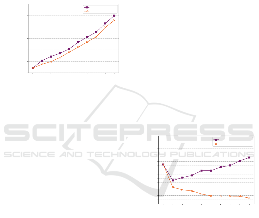
Figure 4: The evaluation of the routing quality.

topology. The left y-axis, related to the Schedule SPT

and Schedule ILP lines, represents the duration of the

part of the integration cycle used for the TT communi-

cation and the right y-axis, related to the New link ILP

and New link SPT line, represents the volume of the

data exchanged through the newly introduced links.

As can be observed from “Schedule SPT” and

“Schedule ILP” lines in Fig. 4, adding nine additional

edges to the tree topology can shorten the duration of

the part of the incremental cycle used by the TT com-

munication to almost 50%. However, the beneﬁts of

the redundant links is that it can utilize the proposed

method based on the MILP model (labeled as “Sched-

ule ILP” in the ﬁgure) better than the method based on

the SPT algorithm. On the tree topology, both meth-

ods behave equally as the routing tree is already de-

cided by the topology. However, as the number of ad-

ditional links is increasing, the proposed method acts

signiﬁcantly better than the SPT method.

The “New link” lines, on the other hand, shows

how the signiﬁcance of the newly introduced links

evolves with the number of additional edges in the

topology. The routing algorithms are able to forward

through the last added message only about one-third

of the data volume compared to the data volume it was

able to forward through the ﬁrst added link.

4.2 Impact of the Incremental

Scheduling on the Schedule

The backward compatibility constraint introduced to

the scheduling problem causes the overhead in the

resulting schedule. To measure the overhead of

the incremental scheduling over the non-incremental

scheduling, another experiment was performed. The

new set of benchmark instances was generated with

ten incremental iterations. In the case of the incre-

mental scheduling, the resulting schedule from the

previous iteration was used as the original sched-

ule. The ﬁrst incremental scheduling iteration has an

empty original schedule. All the messages were gen-

Incremental Scheduling of the Time-triggered Trafﬁc on TTEthernet Network

309

erated with a period in a range from one to three inte-

gration cycles and with Ethernet frame lengths in full

range. The last incremental iteration instances con-

tained 500 TT messages.

The results from the experiment are presented in

Fig. 5. The incremental scheduling iteration is sit-

1 2 3 4 5 6 7 8 9 10

Incremental scheduling iteration

200000

250000

300000

350000

400000

450000

500000

Part of the integration cycle

used by TT communication [ns]

Incremental

Non-incremental

Figure 5: The difference between the incremental and non-

incremental scheduling.

uated on the x-axis of the graph, and the schedule

duration of the part of the integration cycle used by

TT communication is on the y-axis. The dark purple

row represents the result from the algorithm where the

original schedule is considered, while the orange row

represents the results of the algorithm, assuming no

original schedule is given.

The result for the ﬁrst incremental iteration is the

same for incremental and non-incremental scheduling

as no original schedule is used and, consequently, no

backward compatibility constraint is applied in both

cases. The most notable change in the difference be-

tween the incremental and non-incremental schedul-

ing is present in the second incremental iteration. The

prolongation caused by new messages in the case of

the incremental scheduling is almost twice as much

compared to the prolongation caused by the new mes-

sages in the case of the non-incremental scheduling.

This causes the fact that the messages that were al-

ready scheduled in the ﬁrst incremental iteration can-

not be moved in the incremental scheduling. Thus,

the new messages cannot be incorporated in such an

efﬁcient way as in the case of the non-incremental

scheduling. However, this overhead also introduces

a new porosity to the schedule. The further incremen-

tal scheduling iterations are able to use this porosity to

place the new signals into those gaps efﬁciently. That

is the reason why the overhead stays almost constant

in the future scheduling iterations, and the difference

between the incremental and non-incremental sched-

ule is almost the same as can be observed in the graph.

4.3 Evolution of the Schedule

Utilization Over Incremental

Iterations

To support the statement from the previous section,

the way how the utilization of the schedule evolves

with the incremental iterations has been studied more

deeply. For the purpose of this section, the utilization

of the schedule (or just utilization) is deﬁned as the

portion of the part of the integration cycle used for

the TT communication that is utilized by the message

transmission averaged over all the integration cycles.

In other words, considering only the part of the in-

tegration cycle used by the TT communication, the

utilization represents the portion of the time when the

link is busy. In order to test the utilization, similar

benchmark instances were generated to the testing of

the impact of the incremental scheduling. The only

exception is the topology of the network. To avoid

the impact of the routing on the porosity test, the gen-

erated instances use a tree topology. Two different

measurements were performed.

Firstly, the average of the schedule utilization over

the whole network (all the links) has been measured.

The resulting graph can be seen in Fig. 6. The ﬁgure

1 2 3 4 5 6 7 8 9 10

Incremental scheduling iteration

23.0

23.5

24.0

24.5

25.0

25.5

26.0

26.5

27.0

27.5

28.0

28.5

29.0

29.5

Average link porosity

over whole network [%]

Untouched topology

Augmented topology

Figure 6: The average utilization of the communication over

the whole topology.

presents the evolution for two cases: the dark purple

line shows how the utilization evolves when the topol-

ogy is not extended during the incremental iterations;

the orange line shows the utilization evolution when

the topology grows together with the number of mes-

sages. The x-axis represents the incremental schedul-

ing iteration, and the y-axis represents the average

utilization of the schedule in percent. This unuti-

lized/free space can be used by the new messages in

the future incremental scheduling iteration that are lo-

cal (their transmitter and receivers are close to each

other according to the network topology). Note that

ICORES 2022 - 11th International Conference on Operations Research and Enterprise Systems

310

less than 30 % of the schedule is used according to the

graph. This small amount is caused by the tree topol-

ogy, where the links close to the leaves of the topology

are rarely used. The ﬁgure also shows that the overall

schedule utilization increases if there is no topology

extension which is caused by adding new messages to

the schedule and the signiﬁcant part of them are lo-

cal messages (thus, the part of the integration cycle

used by the TT communication is not prolonged too

signiﬁcantly). If the topology is extended, the new

sparse links introduce a lot of unutilized bandwidth to

the schedule, which causes a decrease in the overall

utilization.

Opposed to the new local messages that, as can be

observed from Fig. 6, can be easily incorporated into

the schedule without prolongation of the part of the

integration cycle used by TT communication because

of the low utilization of the links close to leaves, the

new messages that need to transit the root node could

cause the prolongation of the part easily. To study

how the schedule utilization can impact the schedul-

ing of these messages, the second measurement was

performed where the utilization was calculated only

on the most utilized link.

1 2 3 4 5 6 7 8 9 10

Incremental scheduling iteration

Utilization of the most utilized link [%]

Augmented topology

Untouched topology

Figure 7: The porosity of the most utilized link.

The utilization of the most utilized link is pre-

sented in Fig. 7. Here, the utilization is about 77

to 86 %, depending on the particular incremental

scheduling iteration. This makes it harder to incor-

porate the long-distance messages efﬁciently into the

schedule without prolongation of the part of the in-

tegration cycle used by the TT communication. The

ﬁgure also shows that there is no signiﬁcant difference

for the long-distance messages, whether the topology

is extended (but no cycles introduced) or not as the

topology does not inﬂuence the ﬂow of the messages

over the most utilized link.

These graphs also support the statement from the

last section as both the utilization metrics are the

worst in the ﬁrst incremental scheduling iteration,

making the second scheduling iteration the most difﬁ-

cult. After that, the utilization metric changes slowly

and, thus, the difference between the efﬁciency of the

incremental and non-incremental scheduling is simi-

lar.

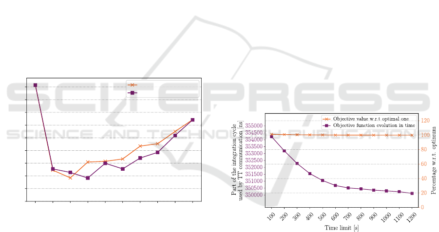
4.4 Evolution of the Scheduling

Objective Function in Time

It is necessary to note that the optimal solution for

the routing algorithm, together with the optimal solu-

tion for the link scheduling algorithm, does not ensure

the optimal solution from the problem statement point

of view. Thus, in practical cases, it is not needed to

wait until the link scheduling algorithm proves that

the current solution is optimal (or close to optimum

in the case of the 1 % tolerance), and the search can

be stopped sooner. This allows for creating sched-

ules for bigger industrial size instances in a reason-

able time. To show how the duration of the part of

the incremental cycle used by the TT communication

evolves in time, the same benchmark instance set with

2000 messages was used. The evolution of the dura-

tion of the part of the incremental cycle used by the

TT communication during the link schedule creation

is presented in Fig. 8.

Figure 8: The evolution of the duration of the part of the in-

cremental cycle used by the TT communication in the time

domain.

The x-axis of the ﬁgure represents the time limit

for the scheduling. At the time of 1200 s, all the in-

stances in the set were solved to optimality. The left

y-axis represents the average duration of the part of

the integration cycle used by the TT communication

over the whole benchmark set. The left y-axis rep-

resents the ratio of the obtained objective value at a

particular time compared to the optimal one in per-

centage. Until time 100 s, the scheduling algorithm

was not able to ﬁnd a feasible solution for two in-

stances out of thirty. At time 200 s, there was only

one instance without ﬁnding a feasible solution. In all

Incremental Scheduling of the Time-triggered Trafﬁc on TTEthernet Network

311

further times, all the instances have found a solution.

The major change in the duration occurs in the be-

ginning, and the slope is decreasing in time. Even if

there is some improvement in the average duration of

the part of the integration cycle used by the TT com-

munication during the whole scheduling period, the

improvement between the average duration obtained

at time 100 s and 1200 s is less than 1.3 %. Thus, it

is sufﬁcient to use a solution, which is not necessar-

ily optimal from the link schedules creation problem

point of view but obtained in a shorter time, in many

practical cases.

4.5 Scheduling of the Real Industrial

Instances

The work has been motivated by our industrial part-

ner, who develops electronic systems for the avionic

industry. This section describes the behavior of the

proposed algorithm on the real instance obtained from

the partner. The instance contains 1922 messages

(407 unicast messages and 1515 multicast messages)

with a payload of up to 1036 bytes and periods

from the set {12.5 ms, 25 ms, 50 ms, 100 ms, 200 ms,

1000 ms}. The system consists of 38 nodes. The

topology is based on three switches SW1, SW2 and

SW3 that are mutually interconnected. Each such

switch is in the topology twice called SW1 A and

SW1 B, and these two instances are interconnected

too. Thus, the backbone of the network is based on

such a double triangle topology. Each endpoint is

connected to one of those switches. The schedule

for this instance, which is optimal from all the sub-

problem’s point of view, was obtained after less than

250 s. The schedule utilization of the most utilized

link reached 96.3% while the schedule utilization av-

eraged over the whole network was only 19.6%. This

shows that the integration cycle assignment was able

to distribute the messages in the most utilized link

very efﬁciently. Figure 9 presents how the payload is

distributed among the links in the network. The links

are classiﬁed according to the volume of the TT data

transmitted through them per second. The ﬁrst class

includes links with the volume from 0 to 0.1 MB/s, the

second one includes the links with the volume from

0.1 to 0.2 MB/s, etc. The y-axis then represents the

percentage of the links that belong to the particular

class. The histogram shows that almost 70 % of the

links have very low utilization of the links. About

50 % of these links are empty. That means that these

links are connected to the endpoints that serve as a

transmitter or a receiver (note that each transmission

direction of the Full-duplex physical link is repre-

sented by two separate links here). Moreover, there is

0.0

0.1

0.2

0.3

0.4

0.5

0.6

0.7

0.8

Bandwidth of links consumed by the TT traﬃc [MB/s]

Percent of links belonging to

the particular class [%]

65.22

18.12

6.52

3.62

4.35

0.72 0.72 0.72

Figure 9: The histogram of the links utilization.

just one link in the class with 0.7 - 0.8 MB/s. This link

(and also the links from classes with 0.5-0.6 MB/s and

0.6-0.7 MB/s) connects the redistribution node with

the communication endpoint. Thus, the routing al-

gorithm was not able to reroute some messages from

this link through another path to lighten the link. The

backbone links belong to the 0.2-0.3 MB/s and 0.3-

0.4 MB/s classes. The interesting observation is that,

considering the 100 MB/s TTEthernet network, the

TT communication utilizes less than 1 % of the band-

width in this instance. The rest of the bandwidth is

used for the RC and BE communication.

5 CONCLUSION

The pressure placed on, for example, the automotive

or avionics industries to verify and certify its sys-

tems on a component and system integration level

pushes system developers to use time-triggered traf-

ﬁc for safety-related communication as its behavior is

deterministic.

We have followed the idea of separating the time-

triggered trafﬁc and event-triggered trafﬁc already

used in (Dvo

ak et al., 2017), which was inspired by

the scheme of the FlexRay bus communication cycle.

The objective has been to maximize the minimal guar-

anteed coherent gap left in each integration cycle on

each link that can be continuously used by the Rate-

Constrained and Best-Effort trafﬁc while keeping the

backward compatibility with the original schedules

created in the previous development iterations.

The experiments show that the incremental

scheduling on one side prolongs the part of the in-

tegration cycle used by the TT communication in the

order of a percent (in the experiments it was about

1 %), but it brings the advantage of backward com-

patibility. The experiments show that the method can

ICORES 2022 - 11th International Conference on Operations Research and Enterprise Systems

312

return good results even for industry sized instances

in a few minutes. The study of the scalability of the

algorithm dependent on the number of messages, their

length and periodicity is available from the authors of

this paper upon request.

ACKNOWLEDGEMENTS

This work was supported by the EU and the Min-

istry of Industry and Trade of the Czech Republic un-

der the Project OP PIK CZ.01.1.02/0.0/0.0/20 321/

0024399.

REFERENCES

ARINC (Aeronautical Radio, Inc.) (2009). ARINC 664P7:

Aircraft Data Network, Part 7, Avionics Full-Duplex

Switched Ethernet Network. Technical report.

Boyer, M., Daigmorte, H., Navet, N., and Migge, J.

(2016). Performance impact of the interactions be-

tween time-triggered and rate-constrained transmis-

sions in TTEthernet. In 8th European Congress on

Embedded Real Time Software and Syst., pages 159–

168, Toulouse.

Craciunas, S. S. and Oliver, R. S. (2016). Combined task-

and network-level scheduling for distributed time-

triggered systems. Real-Time Syst., 52(2):161–200.

Craciunas, S. S., Oliver, R. S., Chmel

ık, M., and Steiner, W.

(2016). Scheduling real-time communication in IEEE

802.1Qbv time sensitive networks. In RTNS, Brest.

Craciunas, S. S., Oliver, R. S., and Ecker, V. (2014). Opti-

mal static scheduling of real-time tasks on distributed

time-triggered networked systems. In ETFA, pages 1–

8, Barcelona, Spain.

Dvorak, J. and Hanzalek, Z. (2016). Using two indepen-

dent channels with gateway for ﬂexray static segment

scheduling. IEEE Transactions on Industrial Infor-

matics, 12(5):1887–1895.

Dvo

ak, J., Heller, M., and Hanz

alek, Z. (2017). Makespan

minimization of time-triggered trafﬁc on a ttethernet

network. In WFCS, pages 1–10, Trondheim.

International Organization for Standardization (2015).

ISO 17458 - FlexRay communications system.

Kopetz, H., Ademaj, A., Grillinger, P., and Steinhammer,

K. (2005). The time-triggered ethernet (TTE) design.

In ISORC, pages 22–33. IEEE.

Laborie, P. (2017). A (Not So Short) Introduction to CP

Optimizer for Scheduling. In ICAPS.

Li, Z., Wan, H., Pang, Z., Chen, Q., Deng, Y., Zhao, X.,

Gao, Y., Song, X., and Gu, M. (2019). An enhanced

reconﬁguration for deterministic transmission in time-

triggered networks. IEEE/ACM Transactions on Net-

working, 27(3):1124–1137.

Minaeva, A., Akesson, B., Hanzalek, Z., and Dasari, D.

(2018). Time-triggered co-scheduling of computation

and communication with jitter requirements. IEEE

Transactions on Computers, 67(1):115–129.

Moutinho, L., Pedreiras, P., and Almeida, L. (2019). A

real-time software deﬁned networking framework for

next-generation industrial networks. IEEE Access,

7:164468–164479.

Pozo, F., Rodriguez-Navas, G., and Hansson, H.

(2019). Methods for large-scale time-triggered net-

work scheduling. Electronics, 8(7).

SAE International (2011). AS6802: Time-Triggered Ether-

net. Technical report, SAE International.

Steinbach, T., Korf, F., and Schmidt, T. C. (2010). Compar-

ing time-triggered Ethernet with FlexRay: An eval-

uation of competing approaches to real-time for in-

vehicle networks. In WFCS, pages 199–202, Nancy.

Steiner, W. (2010). An Evaluation of SMT-Based Schedule

Synthesis for Time-Triggered Multi-hop Networks. In

RTSS, pages 375–384, San Diego, CA, USA.

Steiner, W. (2011). Synthesis of static communication

schedules for mixed-criticality systems. In ISORCW,

pages 11–18, Newport Beach, CA, USA.

Steiner, W., Gutirrez, M., Matyas, Z., Pozo, F., and

Rodriguez-Navas, G. (2015). Current techniques,

trends and new horizons in avionics networks conﬁg-

uration. In DASC, pages 1–26, Prague.

Tamas-Selicean, D., Pop, P., and Steiner, W. (2015a).

Design optimization of TTEthernet-based distributed

real-time systems. Real-Time Syst., 51(1):1–35.

Tamas-Selicean, D., Pop, P., and Steiner, W. (2015b).

Timing Analysis of Rate Constrained Trafﬁc for

the TTEthernet Communication Protocol. In 18th

IEEE Int. Symp. on Real-Time Distributed Computing,

pages 119–126, Auckland, New Zealand.

Tuohy, S., Glavin, M., Hughes, C., Jones, E., Trivedi, M.,

and Kilmartin, L. (2015). Intra-vehicle networks: A

review. IEEE Transactions on Intelligent Transporta-

tion Systems, 16(2):534–545.

Vlk, M., Brejchova, K., Hanzalek, Z., and Tang, S.

(2022). Large-scale periodic scheduling in time-

sensitive networks. Computers and Operations Re-

search, 137:105512.

Wang, J., Ding, P., Wang, Y., and Yan, G. (2018). Back-

to-back optimization of schedules for time-triggered

ethernet. In 37th Chinese Control Conference (CCC),

pages 6398–6403, Wuhan, China.

Waszniowski, L., Krakora, J., and Hanzalek, Z. (2009).

Case study on distributed and fault tolerant system

modeling based on timed automata. Journal of Sys-

tems and Software, 82(10):1678–1694. SI: YAU.

Incremental Scheduling of the Time-triggered Trafﬁc on TTEthernet Network

313