
Removing Automatically the Ambiguity in Wind Direction Retrieved
from SAR Images
Maria da Conceição Proença
Department of Physics, Marine and Environmental Sciences Centre (MARE-ULisboa), Faculty of Sciences,
University of Lisbon, Campo Grande, 1749-016 Lisboa, Portugal
Keywords: Wind Direction, Wind Shadows, Direction Ambiguity, SAR Images, Image Processing.
Abstract: The evaluation of the wind resource in large areas to study the viability of wind farms is ideally studied using
synthetic aperture radar (SAR) images in which the direction of the wind can be mapped from its effects on
the water surface. Methods in use usually assume a fixed direction from a measurement for the whole image
or interpolate the direction of wind fields from numerical weather models, that can be non-coincident in time
with the SAR snapshot and of much less spatial resolution. The problem remains in the directional ambiguity
of 180 degrees. This work presents three indexes to identify and validate initial “anchor vectors” that could
be used as an aid in the complex process of remove this ambiguity, using wind shadows in the water near the
coastline. These indexes consider several hypotheses to provide for local variability such as physiographic
accidents, the eccentricity of the shadows and the effect of bay-shaped areas, all quantified through image
processing methods. Comparing the results with the reference wind field provided by ESA for the time of
acquisition of the ENVISAT-ASAR image used we could conclude that this is a promising line of work.
1 INTRODUCTION
The ambiguity in wind direction retrieval is a key
problem to which there exists a very recent solution
(
Zhang, 2021) using support vector machine (SVM)
based models, with performance still depending on
sea surface wind speed. The issue of ambiguity has
been addressed from time to time, although wind
direction remains the most appealing problem since
the 1980s (Heron, 1986), (Hildebrand, 1994); later,
(Kerkmann, 1998) mentioned four different methods
for removing the direction ambiguity, all involving a
human operator or a trained meteorologist, one of
them autonomous in the sense that no external data is
needed. In the 2000s two main methods were being
used to wind retrieval – those based on gradient-
oriented histogram (Koch, 2004), and wavelets based
(Du, 2002), (Fichaux, 2002), followed by
improvements from the latter as in (Corazza, 2020),
who use the Radon transform. Some adaptation of
successful methods also took place, like (Horstmann,
2004) who adapts the CMOD4, originally developed
for ERS-1 and 2 to ENVISAT-ASAR images with
success, while (Kerbaol, 2005) uses coastal
information. (Young, 2006) concludes that automatic
and semi-automatic extraction of wind direction are
complimentary and ensure a higher liability in wind
direction retrieval from SAR images. (Koch, 2004) in
the same paper mentioned above uses a
semiautomatic removal of the ambiguity by
combining manual selecting of unique directions on a
set of subimages and automatically choosing the best
aligned directions in the remaining subimages, while
(Song, 2006) uses buoy data to solve the ambiguity in
a comparation of two algorithms for wind speed.
The ambiguity in the direction retrieval was not an
appealing subject for automation, but still seems
possible to implement, at least in areas near the coast.
The image processing methodology exposed here
allowed the identification of anchor vectors near the
shoreline that could act together with global methods
to ensure the wind direction ambiguity is
automatically assessed in the whole wind field, which
could be useful in preliminary studies for offshore
wind farms settings.
2 MATERIALS AND
METHODOLOGY
The image used is a medium resolution synthetic
aperture radar image that was acquired by Envisat
Proença, M.
Removing Automatically the Ambiguity in Wind Direction Retrieved from SAR Images.
DOI: 10.5220/0010934000003209
In Proceedings of the 2nd International Conference on Image Processing and Vision Engineering (IMPROVE 2022), pages 93-100
ISBN: 978-989-758-563-0; ISSN: 2795-4943
Copyright
c
2022 by SCITEPRESS – Science and Technology Publications, Lda. All rights reserved
93
ASAR – Wide Swath Mode (WSM) instrument, with
a nominal resolution of 150x150 m (range x azimuth),
a pixel spacing of 75 m and covering 400X400 km
(https://earth.esa.int) acquired over Corsica at 2007-
11-13 (Figure 1-a).
To make the successive processing steps of the
methodology more perceptible, we will be using the
sub-image identified in red (Figure 1-b) in the
ENVISAT image whenever we consider more useful
that the detail is observed to illustrate the reasoning.
a
b
Figure 1: SAR image acquired by ENVISAT mission over
Corsica (a) and zoom on the area which will be used to
illustrate the image processing operations (b).
The first step involves calibration and
computation of a land mask, and it was achieved with
ESA open-source software Next ESA SAR
Toolbox (NEST). A land mask is a binary image to
discriminate between land and water, with two values
usually 0 and 1), where we can attribute the value 1
to the subject of interest to be altered in subsequent
morphological operations until we have the suitable
mask to apply to the work image.
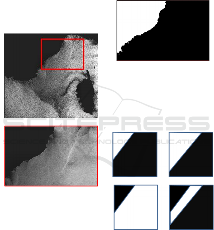
From the land mask obtained (Figure 2), a
sequence of morphological and logical operations is
needed to obtain a “ribbon mask”. The procedure is
schematically detailed in Figure 3.
Figure 2: Land mask obtained using NEST: binary image
where the land is represented with the value 1 (white) and
the sea area has the value 0 (black).
Using the initial land mask here represented by a
white triangle in a black background (Figure 3-a), two
binary images are computed: the first one by dilation,
a morphological operation that enlarge the areas with
value 1 presented in white (Pratt, 2001) to obtain a
new mask (Figure 3-b), and the second one by
inversion: the value 1 in the initial image becomes 0
and vice-versa (Figure 3-c).
a
b
c
d
Figure 3: Schematic representation of the sequence of
operations to obtain a “ribbon” mask: (a) initial land mask,
(b) dilation of (a), (c) inversion or negation of (a) and (d)
logical AND between (b) and (c) – only the areas where
both masks have value 1 will receive a positive value.
IMPROVE 2022 - 2nd International Conference on Image Processing and Vision Engineering
94
The structural element used for dilation in the
ENVISAT image was a disk of radius 25 pixel,
applied successively the number of times needed to
encompass all the area containing shadows – to
automatize this step, a maximum width for the mask
should be assessed from a bigger dataset of images of
the same sensor.
When those masks (Figure 3-b and c) are
combined by a logical AND operation, the result is a
“ribbon mask” (Figure 3-d).
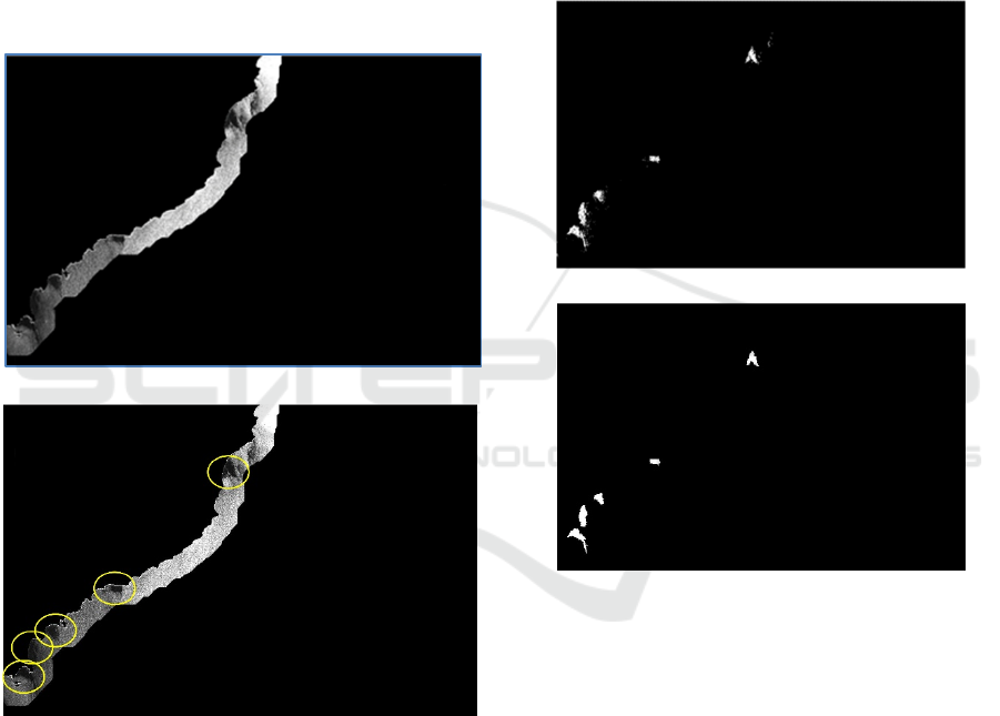
With the new mask a corridor near the coastline
can be isolated (Figure 4-a), where the wind shadows
are now visible as dark spots near the shoreline
(Figure 4-b).
a
b
Figure 4: The “ribbon” mask is applied to the original image
(a), isolating the area of water near the shoreline, where
wind shadows are apparent (b).
Next step is to isolate the shadows as individual
objects, which is made by thresholding the image
(Figure 5-a), giving the value 1 to the pixels that are
between the thresholds 0 (corresponding to the area
masked) and an appropriate radiometric level, that
will depend on the image codification – pixels in 16
bits images are in the range [0, 65 535], while in 8 bits
images only 256 levels are possible, in the range [0,
255]. The threshold is computed using the subset of
pixels belonging to the corridor and assigned to the
average less two standard deviations of the intensities
present.
Once the threshold is applied to the image, the
resulting binary image is ready for the morphological
operations needed to consolidate each shadow, that
will consist in a sequence of dilation followed by
erosion with the same structuring element, usually
called closing (Figure 5-b), achieved with a smaller
structural element to preserve the form - here a disk
of radius 11.
a
b
Figure 5: Candidates for wind shadows isolated by intensity
thresholding (a) and consolidated using morphological
operations (b).
After shadow localization, we looked for the
digital elevation model (from SRTM, characterized
below) to analyse each shadow and its immediate
neighbourhood on land, to determine its credibility as
a wind shadow (Figure 6). Three validation criteria
are proposed: a bay factor, an abrupt cliff analysis and
the shadow eccentricity, detailed and evaluated in the
next section.
Removing Automatically the Ambiguity in Wind Direction Retrieved from SAR Images
95
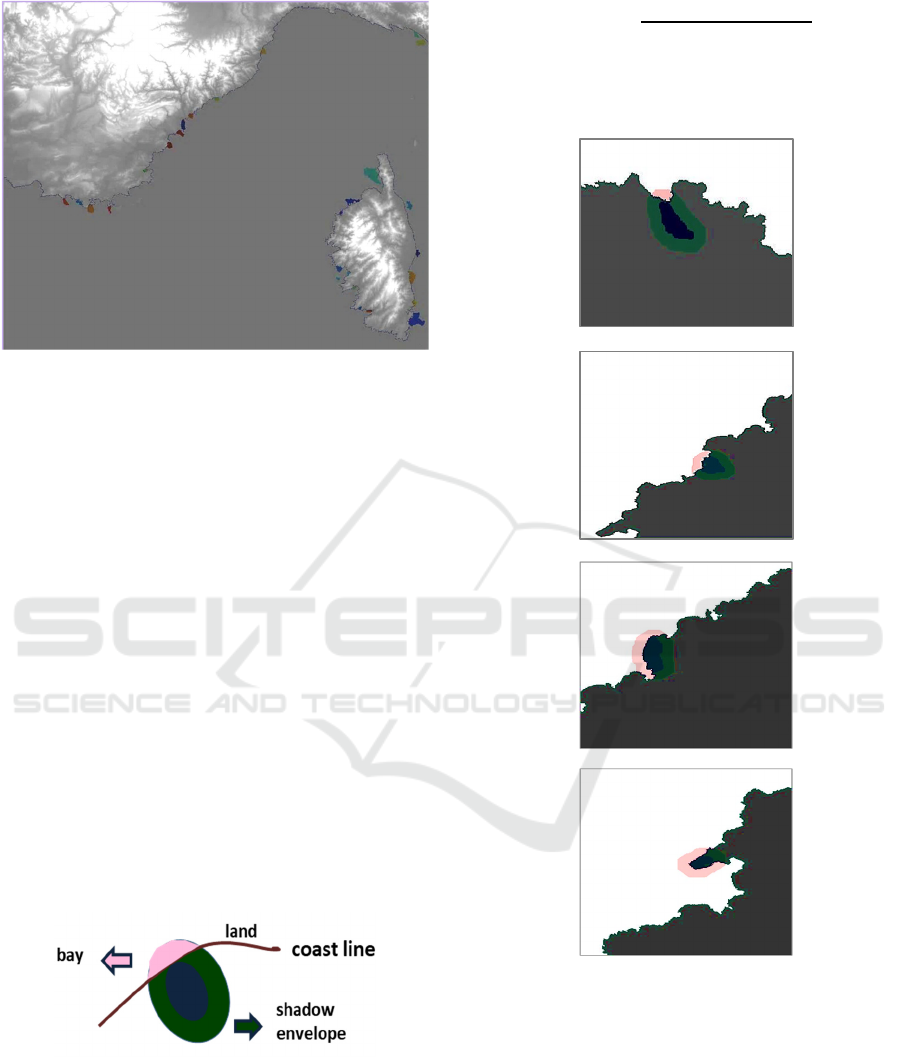
Figure 6: The candidates to wind shadows in different
colours and the digital elevation model on land side.
3 VALIDATION CRITERIA
The criteria proposed for validation of the wind
shadows as such are not exhaustive but worked in the
range of conditions present in the image and can be
applied to any similar coastline, as the three are based
in common physiographic and natural effects.
3.1 Bay Factor
The rationale for the Bay factor sits in the fact that an
open bay will not provoke a wind shadow, while a
more closed bay will usually induce an area of
shadow in the near water.
This was transformed in a quantitative index
using the quotient between the number of pixels that
constitute the bay envelope and the number of pixels
belonging to the shadow envelope, schematically
identified in Figure 7.
Figure 7: Definition of the pixels forming the bay envelope
in pink in the land side, and the pixels belonging to the
shadow envelope, in green, in turn of the blue shadow over
the water.
The Bay factor computed this way (eq. 1) will be
bigger for a closed bay, and low for an open bay.
Bay factor =
∑
,
, ∈
∑
,
, ∈
(1)
Examples of the values obtained for different
forms of bays with this definition and the shadows
previously processed are shown in Figure 8.
a
b
c
d
Figure 8: Examples of shadows and bays present in the
image. Land is white and water is grey, and the bay and
shadow envelopes follow the colour code in Figure 7. The
values for the bay factor are 0.09 (a), 0.28 (b), 0.50 (c) and
0.79 (d).
A very closed bay such as the one in Figure 8-c
will have a high Bay factor, but this configuration
probably is enough cause for a calm water, observed
as shadow in a SAR image, so shadows scoring high
Bay factors will not be considered wind shadows.
IMPROVE 2022 - 2nd International Conference on Image Processing and Vision Engineering
96
3.2 Abrupt Cliff Index
The altimetry came from the digital elevation data
(DEM) obtained by the Shuttle Radar Topography
Mission (SRTM), an international project
spearheaded by the U.S. National Geospatial-
Intelligence Agency (NGA) and the U.S. National
Aeronautics and Space Administration (NASA). The
project covered more than 80% of the Earth’s solid
surface during a 11-day mission of the Space Shuttle
Endeavour in February 2000. The SRTM data is
available as 3 arc second (approx. 90 m ground
resolution) and has a vertical error reported to be less
than 16 m (https://www.usgs.gov).
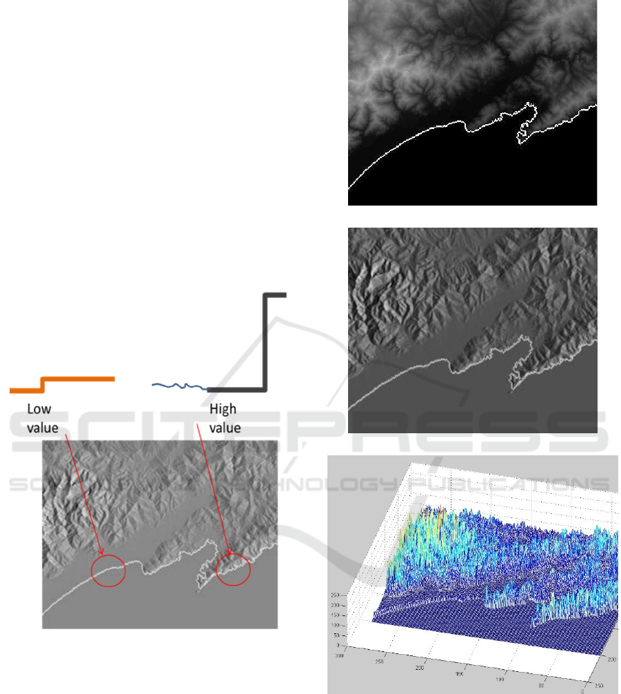
This digital elevation model was used to compute
the local gradient near each shadow. A flat area will
have a low local gradient, and a steepest area will
have a higher value (Figure 9).
Figure 9: The flat area on the left will have a low value for
the local gradient while the abrupt cliffs on the right will
have a high gradient.
The cliff index is computed considering the local
elevation from the DEM (Figure 10-a), its gradient
(Figure 10-b), and the absolute value of this gradient
(Figure 10-c). The roughness of the terrain becomes
more apparent with these operations.
The ACliff index is the sum of the pixels
belonging to the seashore shadow track (sst) in the
image containing the absolute value of the gradient of
the elevation (eq. 2).
ACliff =
∑
absgradelevation ))
,∈
(2)
a
b
c
Figure 10: The sequence of images needed to compute the
Abrupt Cliff index: the local elevation from the DEM (a),
the gradient of the local elevation (b) and its absolute value
(c).
As the terrain becomes steeper, the abrupt cliff
index increases. When a shadow is near a flat area
(Figure 11-a), the cliff index will be low, and will
increase as the terrain roughness increases.
Removing Automatically the Ambiguity in Wind Direction Retrieved from SAR Images
97
a
b
c
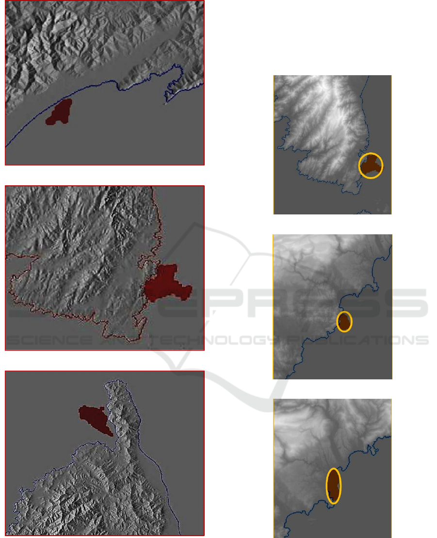
Figure 11: Examples of three shadows (red) near terrain
with different characteristic – the CliffIndex is 1.1 for flat
terrain (a), 4.8 for the shadow near median elevation (b),
and 11.4 for the shadow near abrupt cliffs (c).
3.3 Shadow Eccentricity
The last indicator we consider for the localization of
wind shadows is the eccentricity, computed as the
eccentricity of the ellipsoid enveloping the shadow,
as demonstrated in Figure 12.
a
b
c
Figure 12: Three shadows with different eccentricity values
associated: a) 0.49, b) 0.69 and c) 0.93.
IMPROVE 2022 - 2nd International Conference on Image Processing and Vision Engineering
98
The eccentricity of the ellipsoid is computed as
the square root of the difference between the squared
values of the lengths of the semi-major axis (a) and
semi-minor axis (b) divided by the first (eq. 3).
Eccentricity =
(3)
The information needed is the direction of the
anchor vectors, that will be established from the
centre of the shadows accepted (end point for the
vector) and the nearest point in the coastline,
considering the extension in contact with the ellipsoid
enveloping the shadow (initial point for the vector).
The magnitude of these vectors will be dependent of
the wind field local intensity, and is usually computed
automatically (Rufenach, 1998) since late 90’s.
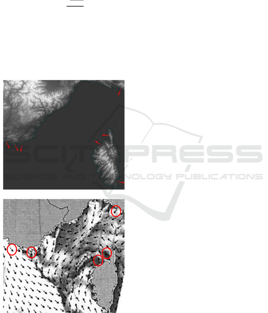
a
b
Figure 13: The seven anchor vectors built from the wind
shadows in the SAR image (a) and the reference wind field
for that date (b).
With these tree indicators, we build a criterion to
accept/reject each candidate shadow as a trustful wind
shadow, with a rationale including a high Cliff index
to identify abrupt cliffs in the proximity of each
shadow that can be the leading cause of the wind
shadow, a low Bay factor to eliminate shadows in
almost enclosed bay areas, and the eccentricity of the
ellipses to refine admissible shadows and find the
line-of-sight in the direction of the shadow to give an
orientation for the anchor vector.
All these criteria and previous location of areas of
interest can be automatically implemented in a single
procedure, avoiding external data and human curation
with inherent subjectivity. To do so, the estimation of
the areas containing shadows can be done with a fixed
maximum width for the ribbon mask.
From the 28 shadow candidates, only 7 verify the
criteria (Figure 13-a).
Considering the positioning of the seven vectors
obtained from the wind shadows and comparing with
the wind vectors in approximately the same positions
in the reference wind field provided by ESA for that
date (Figure 13-b), we can see the orientation of the
seven vectors agree in a reasonable extend with the
local orientation of the wind field.
4 CONCLUSIONS
Wind field monitoring is especially important in the
preliminary phase to select among the best locations
for wind farms and becomes more difficult when
offshore wind farms are the goal.
This case study intended to show that SAR images
allow to directly extract sets of vectors near the
coastline that could be used to unwrap the wind
direction ambiguity in large areas automatically,
complementing the wind direction retrieval that is
already automatized, with a reasonable confidence.
With this kind of procedure, all the operations for
wind retrieval offshore could be completed without
the need of in-situ data (buoy or other external data),
directly from the remote sensed images.
ACKNOWLEDGEMENTS
Envisat-ASAR image and reference wind field were
both courtesy of Alexis Mouche, with CLS at the
time.
Removing Automatically the Ambiguity in Wind Direction Retrieved from SAR Images
99

REFERENCES
Zhang, Y., Chen, X., Meng, W., Yin, J., Han, Y., Hong, Z.,
Yang, S. (2021). Wind Direction Retrieval Using
Support Vector Machine from CYGNSS Sea Surface
Data. In Remote Sens. 2021, 13, 4451.
Heron, M., Rose, R. (1986) On the application of HF ocean
radar to the observation of temporal and spatial changes
in wind direction. In IEEE J. Ocean. Eng. 11(2), pp.
210-218.
Hildebrand, P.H. (1994) Estimation of sea-surface winds
using backscatter cross-section measurements from
airborne research weather radar. In IEEE Trans.
Geosci. Remote Sens. 32, 110–117.
Koch, W. (2004) Directional analysis of SAR images
aiming at wind direction. In IEEE Trans. Geosci.
Remote Sens. 42, pp. 702–710.
Du, Y., Vachon, P. W., Wolfe, J. (2002) Wind direction
Estimation from SAR images of the Ocean Using
Wavelet Analysis. In Can. J. Remote Sens. 28, pp. 498-
509.
Fichaux, N., Ranchin, T. (2002) Combined extraction of
high spatial resolution wind speed and wind direction
from SAR images: A new approach using wavelet
transform. In Can. J. Remote Sens. 28, pp. 510–516.
Corazza, A., Khenchaf, A., Comblet, F. (2020) Assessment
of Wind Direction Estimation Methods from SAR
Images. In Remote Sens. 12.
Horstmann, J., Koch, W., Lehner, S. (2004). Ocean wind
fields retrieved from the advanced synthetic aperture
radar aboard ENVISAT. Ocean Dynamics, 54 (6) :570-
576.
Kerbaol, V., Collard, F. (2005). SAR-derived coastal and
marine applications: From research to operational
products. In Ieee Journal Of Oceanic Engineering, 30
(3), pp. 472-486.
Young, G. S., Sikora, T. D., Winstead, N.S. (2006) Manual
and Semiautomated Wind Direction Editing for Use in
the Generation of Synthetic Aperture Radar Wind
Speed Imagery, J. Applied Meteor. and Climatology,
46, pp. 776-790.
Song, G., Hou, Y., He, Y. (2006) Comparaison of two wind
algorithms of ENVISAT ASAR at high wind, Chin. J.
of Oceanology and Limnology, 24(1), pp. 92-96.
Kerkmann, J. (1998) Review on ScatterometerWinds,
EUMETSAT Tchn. Memorandum N.3, Chap. 6.
https://earth.esa.int/ Available online: ASAR Products
Information - Earth Online (esa.int), (accessed on
07/11/2021).
W. K. Pratt (2001) Digital image processing. Ed. J. Wiley
& Sons, 3rd edition.
https://www.usgs.gov Available online: USGS EROS
Archive - Digital Elevation - SRTM Mission Summary
| U.S. Geological Survey, (accessed on 07/11/2021).
Rufenach, C. (1998) Comparison of Four ERS-
1 Scatterometer Wind Retrieval Algorithms with Buoy
Measurements, J. Atm and Oceanic Technology, 15, pp.
304-313.
IMPROVE 2022 - 2nd International Conference on Image Processing and Vision Engineering
100
