A Comprehensive Study of Vision Transformers on Dense Prediction

Tasks

Kishaan Jeeveswaran, Senthilkumar Kathiresan, Arnav Varma, Omar Magdy, Bahram Zonooz

and Elahe Arani

Advanced Research Lab, NavInfo Europe, Eindhoven, The Netherlands

Keywords:

Vision Transformer, Convolutional Neural Networks, Robustness, Texture-bias, Object Detection, Semantic

Segmentation.

Abstract:

Convolutional Neural Networks (CNNs), architectures consisting of convolutional layers, have been the stan-

dard choice in vision tasks. Recent studies have shown that Vision Transformers (VTs), architectures based on

self-attention modules, achieve comparable performance in challenging tasks such as object detection and se-

mantic segmentation. However, the image processing mechanism of VTs is different from that of conventional

CNNs. This poses several questions about their generalizability, robustness, reliability, and texture bias when

used to extract features for complex tasks. To address these questions, we study and compare VT and CNN

architectures as a feature extractor in object detection and semantic segmentation. Our extensive empirical

results show that the features generated by VTs are more robust to distribution shifts, natural corruptions, and

adversarial attacks in both tasks, whereas CNNs perform better at higher image resolutions in object detection.

Furthermore, our results demonstrate that VTs in dense prediction tasks produce more reliable and less texture

biased predictions.

1 INTRODUCTION

CNNs’ remarkable performance has made them the

prominent choice of architecture in computer vision

tasks (He et al., 2016; Tan and Le, 2019). On the

other hand, the Transformers have become dominant

in NLP owing to their ability to learn long-term de-

pendencies via self-attention. Recent breakthrough of

VTs (Dosovitskiy et al., 2020) demonstrated that the

Transformer-based architecture can also be applied to

image classiﬁcation. This motivated the vision com-

munity to adapt the self-attention based architectures

as feature extractors for more complex tasks such as

depth prediction (Ranftl et al., 2021), object detec-

tion, and semantic segmentation (Liu et al., 2021;

Srinivas et al., 2021). VTs have achieved compelling

performance in these tasks, presenting them as an al-

ternative architectural paradigm.

However, the mechanism by which VTs process

the images is signiﬁcantly different from that of well-

studied CNNs. CNNs use a sequence of convolutional

layers to extract features with progressively increas-

ing receptive ﬁeld. These convolutional layers have

inherent inductive biases, such as locality and transla-

tion equivariance, that are helpful for computer vision

tasks. However, their local receptive ﬁeld makes them

incapable of capturing the global context. VTs, on the

other hand, split the input image into non-overlapping

tokens, and use a sequence of self-attention modules

to process these tokens. These self-attention modules

have global receptive ﬁeld, but they lack the inductive

biases inherent in convolutional layers, making them

data hungry. Therefore, the choice of these two archi-

tectures comes with their own merits and limitations.

The difference in the fundamental working prin-

ciples of VTs compared to CNNs raises many ques-

tions: How well do they perform for distribution

shifts? How robust are they to the adversarial attacks?

How reliable are their predictions for real-world ap-

plications? To what extend they learn the shortcuts,

such as the texture of an object, rather than the in-

tended solution? Although few of these questions are

addressed in the image classiﬁcation domain (Bho-

janapalli et al., 2021; Paul and Chen, 2021), they have

not yet been fully addressed for complex tasks in-

cluding detection and segmentation. To this end, we

perform an in-depth analysis by constructing simple

detection and segmentation models using DeiT (Tou-

vron et al., 2020) as the feature extractor for dense

prediction tasks. Our contributions are as follows:

Jeeveswaran, K., Kathiresan, S., Varma, A., Magdy, O., Zonooz, B. and Arani, E.

A Comprehensive Study of Vision Transformers on Dense Prediction Tasks.

DOI: 10.5220/0010917800003124

In Proceedings of the 17th International Joint Conference on Computer Vision, Imaging and Computer Graphics Theory and Applications (VISIGRAPP 2022) - Volume 4: VISAPP, pages

213-223

ISBN: 978-989-758-555-5; ISSN: 2184-4321

213

Transformer

Encoder

N embeddings

Image

N, 16x16 patches

Reshape

CCCC IIII

I I I I

FM1

FM2 FM3

FM4 FM5

H/4 X W/4 X 256

H X W X N

FCOS Head

FM1

FM2 FM3 FM4 FM5

Per Pixel

Classification

Bbox +

Classification

Segmentation

Head

Object Detection

Head

DDDI

FM1 FM2 FM3 FM4 FM5

64 X 64 X K

32 X 32 X K

16 X 16 X 512

8 X 8 X 512

4 X 4 X 512

Interpolate

Downsample

Concatenate

...

Patch Embedding

Class token

Distillation

token

Position

Embedding

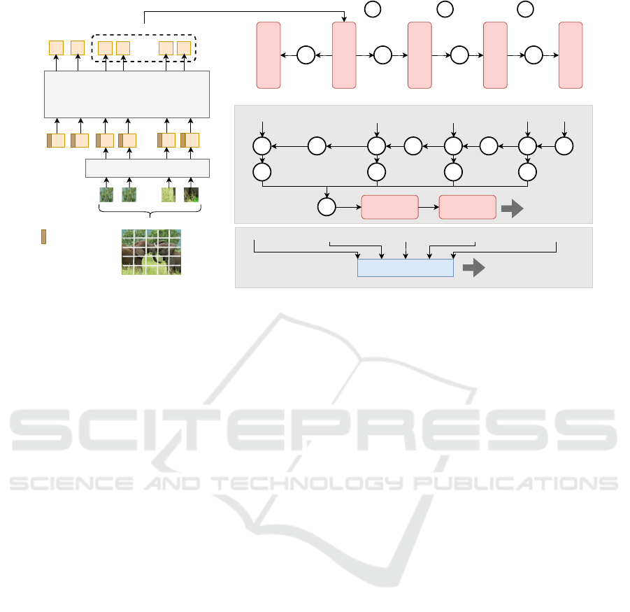
Figure 1: Architecture for object detection and semantic segmentation with VT backbone.

• Evaluating on in-distribution-dataset, we ﬁnd VTs

are more accurate but slower than CNNs coun-

terparts. In addition, the results on out-of-

distribution (OOD) dataset reveals that VTs are

also more generalizable to distribution shift.

• Our results show that VTs are better calibrated

and thus, more reliable than CNNs, thereby mak-

ing them better suited for deployment in safety-

critical applications.

• Increasing the inference image resolution, we

show that the performance of both VTs and CNNs

degrade. However, in detection, CNNs outper-

form their VT counterparts at higher resolutions.

• We demonstrate that VTs converge to wider min-

ima compared to CNNs, which we attribute to

their generalizability.

• We show that VTs are consistently more robust

to natural corruptions and (un)targeted adversarial

attacks than CNNs.

• We extend the texture bias study (Bhojanapalli

et al., 2021) for dense prediction tasks. The re-

sults show that the VTs are less dependent on tex-

ture cues than CNNs to make their predictions.

2 RELATED WORK

Transformer architectures adapted for image classi-

ﬁcation, such as ViT (Dosovitskiy et al., 2020) and

DeiT (Touvron et al., 2020), have achieved compa-

rable performance to state-of-the-art CNNs. Later

methods modiﬁed these vision transformers(VTs) to

act as feature extractors in dense prediction tasks such

as object detection, semantic segmentation, and depth

prediction (Wang et al., 2021; Liu et al., 2021; Ranftl

et al., 2021). The progress of VTs present them as an

alternative architecture to CNNs across vision tasks.

To study the impact of architecture change, re-

cent works have compared VTs and CNNs on as-

pects beyond speed and accuracy for image classiﬁ-

cation. Among these works, studies such as (Bho-

janapalli et al., 2021) and (Paul and Chen, 2021) have

compared VTs and CNNs in terms of robustness to

adversarial attacks and natural corruptions. (Naseer

et al., 2021) further studied the texture-bias of VTs

and CNNs for image classiﬁcation. (Minderer et al.,

2021) additionally investigated the model calibration

of VTs and CNNs, and demonstrated that type of ar-

chitecture is a major determinant of properties of cal-

ibration. However, there has been no study of the im-

pact of VTs on generalizability, robustness, calibra-

tion, and texture-bias in dense prediction tasks, in-

cluding detection and segmentation, when replacing

CNNs as the feature extractor.

We perform an exhaustive comparison of VTs and

CNNs for their generalizability to higher resolutions

and distribution shifts, robustness to adversarial at-

tacks and natural corruptions, reliability, and texture-

bias for object detection and semantic segmentation.

3 METHODOLOGY

We conduct the comprehensive empirical study on ob-

ject detection and semantic segmentation tasks with

CNN and VT backbones of different sizes. Here, we

VISAPP 2022 - 17th International Conference on Computer Vision Theory and Applications

214

explain the details of architecture used in this study.

3.1 Transformer as a Feature Extractor

We use Data Efﬁcient Image Transformer (DeiT)

(Touvron et al., 2020) as our VT feature extrac-

tor. In DeiT, the input image is divided into N non-

overlapping patches of a ﬁxed size (16 × 16) and

the patches are ﬂattened and embedded using a lin-

ear layer to K dimensions. A position embedding

is added element-wise to the patch embeddings to

help the model to understand some notion of the or-

der of the input patches. The resulting tensor is

given as input to repeated blocks of self-attention and

feedforward layers. The ﬁnal representation of class

encoding is passed through a feedforward network

(FFN) before feeding it to a softmax layer to infer

the classes. The class encoding learns the context and

class speciﬁc information from the image patches.

We modify DeiT to make it suitable for object de-

tection and semantic segmentation by removing the

FFN and reﬁning the outputs of the ﬁnal block (N +2

embeddings) before passing on to the heads. The re-

ﬁnement process includes removing the class and dis-

tillation embeddings (used in DeiT for classiﬁcation)

after which N embeddings remain. These N embed-

dings are reshaped into a feature map of 32 × 32 × K

(FM2 in Figure 1). A series of convolutional down-

sampling layers are used to create multiple feature

maps of spatial dimensions 16 (FM3), 8 (FM4), and

4 (FM5) from FM2. Finally, FM2 is upsampled to

obtain a feature map of spatial dimension 64 (FM1).

These ﬁve feature maps are then passed to the predic-

tion head of the models.

3.2 Detection Head

For object detection, we use Fully Convolutional

One-Stage object detector (FCOS) (Tian et al., 2019),

an anchor-free method that makes predictions based

on key-point estimation, and is one of the state-of-the-

art methods. The detection head infers the classiﬁca-

tion score, bounding box parameters, and centerness

score, and is shared between feature maps at multiple

scales (FM1 to FM5) as shown in Figure 1. Since it

is a pixel-wise dense bounding box predictor, the cen-

terness score is used to suppress low quality bounding

boxes which are predicted at pixel locations far away

from the object center.

3.3 Segmentation Head

For segmentation, the outputs of the backbone are

passed to a light-weight segmentation head to infer

dense pixel-wise classiﬁcation scores. In the seg-

mentation head, starting from the smallest spatial res-

olution, every feature map is interpolated and con-

catenated in the channel dimension with the adjacent

larger feature map. The same approach is adopted for

the subsequent feature maps. These feature maps are

bilinearly interpolated to one-fourth of the input res-

olution, and concatenated. Finally, bilinear interpola-

tion is used to upsample the resultant feature map to

the input resolution, which predicts the class proba-

bilities for every pixel.

4 EXPERIMENTAL SETUP

The experiments are conducted on both detection and

segmentation tasks for VT and CNN backbones of

different network sizes. We use three DeiT variants

as VT backbone - Tiny(T), Small(S), and Base(B)

with input patch size 16×16 - and three CNN counter-

parts with the same range of parameters - ResNet-18

(RN-18), ResNet-50 (RN-50), ResNeXt-101 [32×8d]

(RNX-101).

Training Dataset. The detection models are trained

and evaluated on the COCO dataset (Lin et al., 2014)

which consists of 81 classes. The segmentation mod-

els are trained and evaluated on COCO-Stuff (Caesar

et al., 2018) dataset which contains 172 classes - 80

”things” classes, 91 ”stuff” classes, and 1 unlabelled

class. The datasets consist of 118K training images

and 5K validation images. We choose COCO dataset

for our experiments because it is a challenging bench-

mark dataset with common and naturally occurring

real-world scenes, making it suitable for comparative

experiments on dense prediction models.

Training Details. All models are trained on a Tesla

V100 GPU at 512 ×512 resolution using AdamW op-

timizer (Loshchilov and Hutter, 2019) with an initial

learning rate of 5e

−4

, weight decay of 0.05, and a

cosine learning rate scheduler. The networks with

different backbones are trained with different batch

sizes: DeiT-B and RNX-101 with 8, DeiT-S and RN-

50 with 16, and DeiT-T and RN-18 with 32. The de-

tection models are trained for 55 epochs and the seg-

mentation models are trained for 45 epochs. The data

augmentation includes random horizontal ﬂip, ran-

dom crop, and random photometric distortions such

as random contrast ∈ [0.5, 1.5], saturation ∈ [0.5,1.5]

and hue ∈ [−18,+18]. We use Imagenet (Deng et al.,

2009) pretrained weights for initializing all the back-

bones.

Evaluation Metrics. The metrics used to measure

the performance of segmentation (SEG) and detec-

tion (DET) models are mIoU (mean Intersection over

A Comprehensive Study of Vision Transformers on Dense Prediction Tasks

215

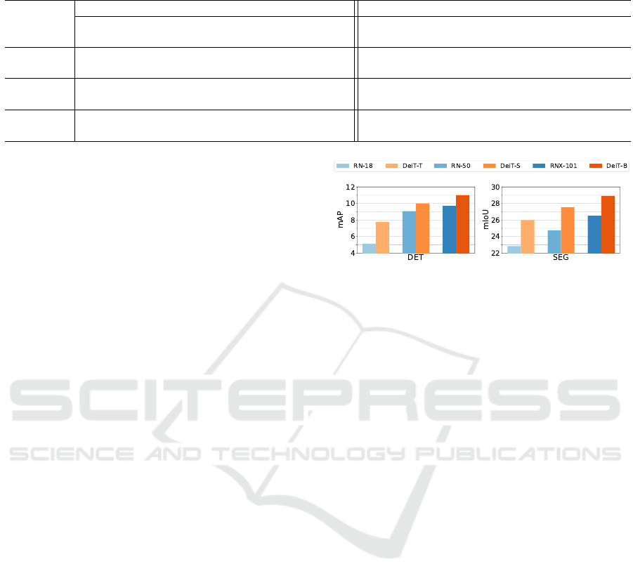
Table 1: Comparison of VTs and their CNN counterparts for object detection on COCO dataset and semantic segmentation

on COCO-Stuff dataset. Best score for each metric is in bold.

Backbone

Detection Segmentation

#Param

(M)

MAC

(G)

Inf.

Time(ms)

mAP

Energy

(kJ)

#Param

(M)

MAC

(G)

Inf.

Time(ms)

mIoU

Energy

(kJ)

RN-18 36 122.34 32.29 26.04 4.6 15 17.76 6.64 30.28 1.7

DeiT-T 30 107.06 41.09 38.19 5.7 11 2.51 11.57 35.08 2.1

RN-50 49 141.00 38.95 39.45 5.3 28 35.02 12.83 35.18 2.4

DeiT-S 49 109.58 46.85 42.56 6.2 28 4.59 18.12 39.79 2.7

RNX-101 114 193.54 60.92 41.20 8.3 93 87.84 27.04 38.02 5.2

DeiT-B 120 116.74 72.33 45.91 9.8 100 12.38 38.14 41.20 6.6

Union) and mAP (mean Average Precision @0.5:0.95

IoU), respectively, unless stated otherwise. In ad-

dition to these accuracy metrics, we report num-

ber of learnable parameters (in millions), Multiply-

Accumulate operations (GMAC) for the architecture,

inference time per image in milliseconds (ms), and

inference energy consumption of a model (in kilo

Joules). We report the average inference time and to-

tal inference energy over 500 samples. All metrics are

calculated at the training resolution.

5 GENERALIZATION

In this section, we probe VTs and CNNs for gener-

alizability to in-distribution and OOD data. We also

investigate the effect of input resolution on general-

ization.

5.1 In-distribution Evaluation

As shown in Table 1, the VT-based object detectors

outperform their CNN counterparts, but at the cost of

inference speed.

Now, MAC represents the computational com-

plexity of the model, and is usually correlated with

the inference speed. Table 1 shows that although VTs

have less complexity than CNNs, they are slower than

CNNs. This might be mainly due to the fact that

GPUs are less optimized for the Transformers (Ivanov

et al., 2020) than CNNs. This could also explain the

higher energy consumption of VTs. Additionally, we

note that the complexity of the largest VTs is less than

that of the smallest CNN (116 vs 122 GMAC). Fur-

thermore, the computational complexity of VTs does

not increase as much as that of CNNs with number of

parameters. Similar to the results for object detection,

the VT-based segmentation models outperform their

CNN counterparts at the cost of inference speed and

energy consumption.

To summarize, VT-based models are more accu-

rate than their CNN counterparts, but the CNN-based

Figure 2: Comparison of VTs and their CNN counterparts

for OOD performance. Object detection models are trained

on COCO and evaluated on BDD100K for 8 classes. Se-

mantic segmentation models are trained on COCO-Stuff

and evaluated on BDD10K for 14 classes.

models are faster and consume less energy. However,

since the VT-based models are less complex, we con-

tend that they can be faster than their CNN counter-

parts if the GPUs are optimized for the VT architec-

tures (Ivanov et al., 2020).

5.2 Out-of-Distribution Evaluation

Despite the good performance of the models on in-

distribution data, it is important to evaluate how well

they perform on unseen data, especially when they

are deployed for real-world applications. The perfor-

mance of the model on such unseen data indicates its

generalizability to OOD datasets.

The detection and segmentation models trained on

COCO and COCO-Stuff are evaluated on BDD100K

(Yu et al., 2020) and BDD10K datasets, respectively.

BDD dataset has a different distribution from that of

COCO since it is composed of road scenes with traf-

ﬁc elements like pedestrians, vehicles, road, and traf-

ﬁc signs. BDD100K for object detection has 10K test

images consisting of 10 classes, out of which, ’rider’

and ’trafﬁc sign’ do not have a corresponding class

in COCO. So, we evaluate the models for 8 match-

ing classes on BDD100K. BDD10K for semantic seg-

mentation, is a subset of BDD100K, with 1k test im-

ages consisting of 19 classes. ’pole’, ’trafﬁc-sign’,

’vegetation’, ’terrain’, and ’rider’ classes do not have

a corresponding class in COCO-Stuff. Thus, we eval-

uate for 14 matching classes and map the COCO-Stuff

VISAPP 2022 - 17th International Conference on Computer Vision Theory and Applications

216

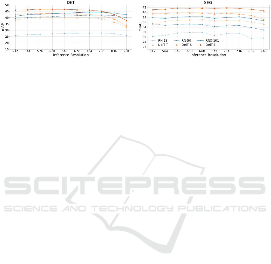
Figure 3: Comparison of VTs and their CNN counterparts at inference resolutions higher than training resolution (512×512).

classes which do not have a corresponding class in

BDD10K to ’unlabeled’ class.

Figure 2 shows that VTs achieve higher perfor-

mance than their CNN counterparts in both tasks.

In segmentation, DeiT-T and DeiT-S also outper-

form signiﬁcantly larger CNN backbones (RN-50

and RNX-101, respectively). Similarly, in detection,

DeiT-S outperforms RNX-101. These results suggest

that the features learned by the VT backbones are

more generalizable to OOD data. We conduct further

experiments in Section 5.4 to analyze the generaliz-

ability of these models.

5.3 Inference Resolution Study

Given the global receptive ﬁeld of VTs (Dosovitskiy

et al., 2020), they should be able to handle larger in-

ference resolutions better than CNNs. Although this

has been tested for depth estimation (Ranftl et al.,

2021), it hasn’t been tested for object detection and

semantic segmentation. Therefore, we compare the

detection and segmentation performance of VT and

CNN backbones when inferred at resolutions higher

than the training resolution (512×512).

When inferring at higher resolutions, the patch

size of VTs is ﬁxed at 16×16 resulting in a larger

sequence length. Though Transformer architectures

can handle arbitrary sequence lengths, VTs need in-

terpolation of the position embeddings to adapt to the

new sequence length. We perform bicubic interpo-

lation over the pretrained position embeddings (Tou-

vron et al., 2020). CNNs, on the other hand, can infer

at higher resolutions without any modiﬁcations.

Figure 3 shows that, in detection, the performance

degradation at higher resolutions is more gradual for

CNNs as compared to VTs. Consequently, CNNs out-

perform their VT counterparts at higher inference res-

olutions in detection. However, this trend is not ob-

served in semantic segmentation, where higher infer-

ence resolution has similar effect on both CNNs and

VTs, and VTs outperform CNNs at all resolutions.

We believe that this is because the interpolated po-

sitional embeddings might not be as effective for de-

tection as they are for segmentation.

Contrary to the conjecture made by (Ranftl et al.,

2021) for depth estimation, the global receptive ﬁeld

of VTs does not provide an advantage over CNNs at

higher inference resolutions for detection. This differ-

ence in behaviour of VTs across tasks raises questions

about the cross-task suitability of interpolating the po-

sition embeddings. We leave this analysis for future

work.

5.4 Convergence to Flatter Minima

Analysis

Since there are multiple solutions to the optimization

objective of a model, the local geometry at the conver-

gence point may affect the model’s generalization. It

has been shown that the models that converge to ﬂatter

minima in the loss landscapes are more robust to dis-

tribution shift, and hence more generalizable (Keskar

et al., 2016; Chaudhari et al., 2019). If models ﬁnd so-

lutions in ﬂatter minima, the performance would not

change signiﬁcantly when the weights are perturbed.

Meanwhile, if the models converge to sharper min-

ima, even a slight perturbation in the weights could

result in drastic changes in performance.

To analyze the generalizability of the trained mod-

els, we add noise with increasing strengths to their

trained weights. The noise is sampled from a Gaus-

sian distribution with mean 0 and standard deviation

ranging from 0.0 to 0.013 in steps of 0.001. Fi-

nally, we infer these models with perturbed weights

on 20% of the training data. As shown in Figure 4,

although performance of all detection and segmen-

tation models degrades as noise increases, VTs per-

form better than CNNs. It is interesting to note that

in detection, DeiT-S and Deit-T have a sharper de-

cline in performance compared to DeiT-B, whereas

in segmentation, all three VTs have a similar decline.

Moreover, in both tasks, the performance of CNNs

degrades much more sharply than that of the VTs,

with the largest CNN backbone (RNX-101) showing

the sharpest drop. Hence, unlike VTs, an increase in

CNN model-size doesn’t necessarily lead to conver-

gence to ﬂatter minima. The results demonstrate that

A Comprehensive Study of Vision Transformers on Dense Prediction Tasks

217

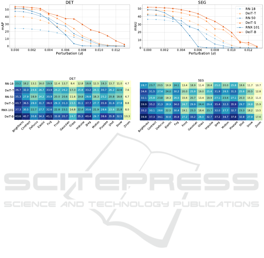
Figure 4: Comparison of train set performance of VTs and their CNN counterparts as a function of Gaussian noise added to

the model parameters.

Figure 5: Performance comparison of VTs and their CNN counterparts under natural corruptions.

VTs converge to ﬂatter minima which could explain

their ability to generalize better to unseen data com-

pared to CNNs as seen in Section 5.2.

6 MODEL CALIBRATION

The neural networks that are being used in safety-

critical applications such as autonomous driving are

expected to be accurate and reliable. Reliable mod-

els are well-calibrated, which means their prediction

conﬁdences and the accuracy of those predictions are

highly correlated. However, recent studies in classi-

ﬁcation have shown that highly accurate CNNs are

poorly calibrated (Guo et al., 2017), and VTs are

better calibrated than CNNs (Minderer et al., 2021).

Here, we extend the reliability study of CNNs and

VTs (Minderer et al., 2021) for detection and segmen-

tation and report the results for in-distribution data.

Expected Calibration Error (ECE) and Maximum

Calibration Error (MCE) (Naeini et al., 2015) are

common metrics used to measure the calibration er-

ror of a neural network in classiﬁcation. ECE is com-

puted by binning the predictions based on the conﬁ-

dence score and taking the weighted mean of the dif-

ference between the average accuracy and conﬁdence

of each bin. MCE, on the other hand, is the max-

imum difference between the average accuracy and

conﬁdence across all bins. We use ECE and MCE

with 15 bins to measure the miscalibration in seg-

mentation models. For object detection, Detection-

ECE (D-ECE) and (w)D-ECE (Kuppers et al., 2020)

are used to measure the calibration error. D-ECE ex-

tends ECE by including the bounding box information

such as coordinates and scale of the bounding box as

additional binning dimensions. (w)D-ECE takes the

weighted average of D-ECE scores with respect to

samples in each class. We use 15 bins, conﬁdence

threshold 0.3, and IoU threshold 0.6 in our analysis.

From the results in Table 2, VTs are better cal-

ibrated than their CNN counterparts in both the

tasks. However, there is no relationship observed be-

tween model-size and calibration within either VTs

or CNNs. Hence, in detection and segmentation, the

calibration of a model is mainly determined by its ar-

chitecture, and not by its size. These observations are

in line with the results in image classiﬁcation (Min-

derer et al., 2021).

7 ROBUSTNESS

Models deployed in an ever-changing environment

are exposed to natural transformations resulting from

weather, lighting, or camera noise, as well as mali-

cious transformations designed by adversaries to fool

the network. It is therefore important to evaluate the

robustness of the model to natural corruptions and ad-

versarial attacks, especially for safety-critical applica-

tions such as autonomous driving. Thus, we evaluate

the robustness of VTs and CNNs to natural corruption

and adversarial attacks when used as a feature extrac-

tor in detection and segmentation.

VISAPP 2022 - 17th International Conference on Computer Vision Theory and Applications

218

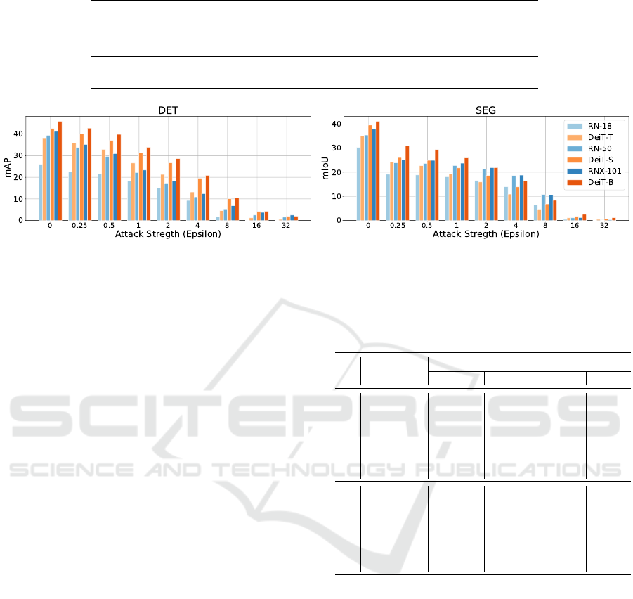
Table 2: Reliability comparison of VTs and their CNN counterparts. Best score for each metric is in bold.

Task Metric RN-18 DeiT-T RN-50 DeiT-S RNX-101 DeiT-B

DET

(w)D-ECE 0.238 0.193 0.200 0.193 0.219 0.165

D-ECE 0.164 0.120 0.145 0.119 0.168 0.094

SEG

ECE 0.157 0.153 0.159 0.158 0.163 0.147

MCE 0.378 0.371 0.389 0.378 0.397 0.369

Figure 6: Performance comparison of VTs and their CNN counterparts under untargeted attack.

7.1 Natural Corruption

To simulate the natural transformations in the real-

world, we apply the 15 common corruptions proposed

by (Hendrycks and Dietterich, 2019) to the valida-

tion set of COCO and COCO-Stuff with severity 3.

We compare the performance of the VTs and CNNs

on the corrupted datasets in Figure 5 and observe

that VTs are more robust than CNNs for both detec-

tion and segmentation. This can be attributed to the

global receptive ﬁeld of self-attention modules in VTs

that help them attend to salient and far away regions,

making them less susceptible to pixel-level changes

caused by corruptions. Figure 7 further provides a

qualitative comparison of the model predictions for

sample corrupted images.

7.2 Adversarial Robustness

An adversarial perturbation is an imperceptible

change in the input image designed to fool the net-

work (Szegedy et al., 2013) into making a particular

prediction (targeted attack) or a wrong prediction (un-

targeted attack). To generate these adversarial exam-

ples, we use the Projected Gradient Descent (PGD)

attack (Madry et al., 2017) on the classiﬁcation loss

for both detection and segmentation. We use a step-

size 1 for min(ε + 4,d1.25εe) iterations, where ε is

the attack strength. We conduct the targeted attack by

swapping ‘person’ and ‘car’ classes.

Figure 6 shows the performance of the models un-

der untargetted attack at varying strengths. In detec-

tion, VTs are more robust to adversarial attacks com-

pared to CNNs at all attack strengths. However, in

segmentation, CNNs are more robust at higher attack

strengths. For the targeted attack, Table 3 shows that

Table 3: Relative performance drop in percentage of VTs

and their CNN counterparts under targeted attack, when

’car’ and ’person’ classes are swapped. Best score for each

metric is in bold. The absolute performances are given in

the Appendix (Table 5).

Backbone

‘Person’ ‘Car’

AP/IoU F1 AP/IoU F1

DET

RN-18 1.88 2.84 11.68 9.00

DeiT-T 1.36 2.62 17.30 12.45

RN-50 1.86 3.01 37.59 12.04

DeiT-S 0.89 2.11 17.76 10.54

RNX-101 2.43 2.91 38.47 9.56

DeiT-B 1.32 2.36 20.86 11.74

SEG

RN-18 20.77 13.22 45.98 36.89

DeiT-T 14.83 9.01 44.59 35.17

RN-50 23.88 15.19 49.61 39.88

DeiT-S 6.94 4.01 20.54 14.32

RNX-101 17.15 10.48 39.08 29.92

DeiT-B 7.81 4.53 15.49 10.63

VTs generally retain a higher percentage of their orig-

inal AP and F1 scores compared to their CNN coun-

terparts. We believe that the adversarial robustness

of VTs, like their robustness to natural corruptions,

can be explained by the global receptive ﬁeld of the

self-attention modules. Moreover, the dynamic na-

ture of the attention modules in VTs makes it harder

for the adversarial attack to ﬁnd successful gradient

directions to fool the network (Khan et al., 2021). Fig-

ure 8 illustrates the predictions by DeiT-S and RN-50

backbones for a sample targeted attacked image.

8 TEXTURE BIAS

Models which learn global shape-related features of

objects are more robust and generalizable than the

A Comprehensive Study of Vision Transformers on Dense Prediction Tasks

219

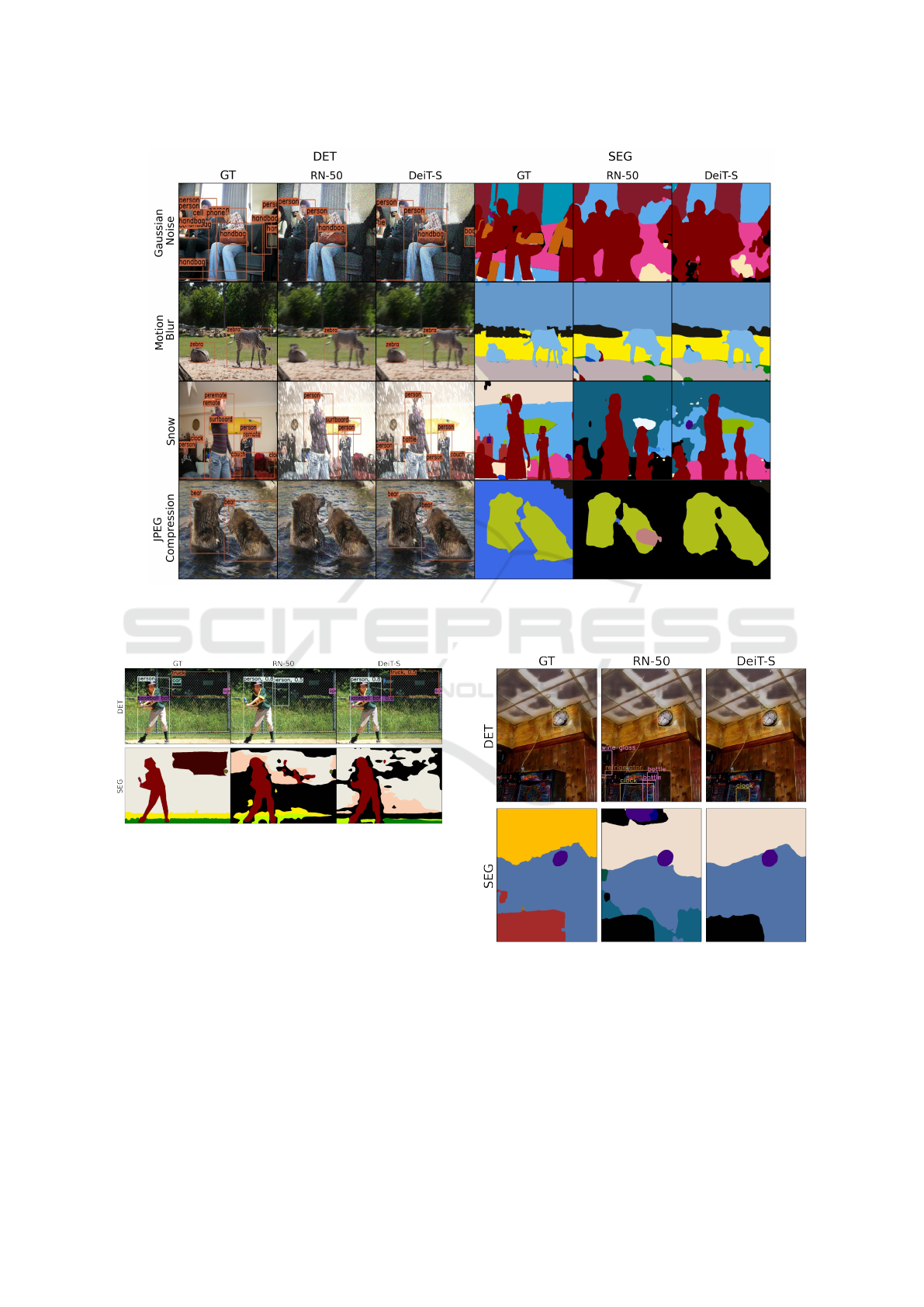
Figure 7: Qualitative comparison of Deit-S and RN-50 predictions on sample corrupted images. CNNs predict the wrong

classes and fail to detect objects more often than VTs. For example, under ‘JPEG Compression’ corruption, RN-50 fails to

detect the objects and predicts a wrong class for part of a region in segmentation.

Figure 8: Qualitative comparison of DeiT-S and RN-50

predictions under targeted attack with ‘person’ and ‘car’

classes swapped. RN-50 predicts ‘person’ class for ‘car’

region in detection and segmentation.

ones which rely on the texture of the objects (Geirhos

et al., 2020). Texture and Shape biases (Hermann

et al., 2020) are used to quantify the relative extent to

which the models are dependent on texture and shape

cues in image classiﬁcation. Here, we extend the tex-

ture and shape bias analyses of VTs and CNNs for

detection and segmentation tasks.

We create a texture-conﬂict dataset of COCO and

COCO-Stuff by applying rich texture from objects

(such as bear and zebra) as a style to other valida-

tion images containing multiple objects of a single

Figure 9: Qualitative comparison of DeiT-S and RN-50 pre-

dictions when the texture of ‘cup’ class is applied on an im-

age. RN-50 predicts ‘bottle’ and ‘wine glass’, which are

under the same super-category as ’cup’ class.

class. A model is said to predict texture in this texture-

conﬂict dataset if it predicts the class of the applied

texture. Similarly, the model is said to predict shape

if it predicts the original class despite the change in

texture. For T texture predictions and S shape predic-

VISAPP 2022 - 17th International Conference on Computer Vision Theory and Applications

220

Table 4: Texture-bias of VT and CNN backbones. SC represents the texture bias based on super-category classes. Best scores

are in bold.

Task SC RN-18 DeiT-T RN-50 DeiT-S RNX-101 DeiT-B

DET

- 4.83 3.10 4.19 2.55 3.54 2.42

X 21.98 20.74 21.35 19.81 21.12 19.06

SEG

- 1.64 1.51 1.78 1.53 1.87 1.65

X 8.42 7.05 8.87 7.39 8.26 6.83

tions, the texture-bias is deﬁned as T /(T + S). From

Table 4, we observe that, unlike in classiﬁcation, the

texture-bias values of the models are low for detection

and segmentation. This is because while the mod-

els do not predict the shape, i.e. the intended class,

they also do not predict the applied texture. However,

from the qualitative analysis in Figure 9, we ﬁnd that

the predictions and the applied-texture belong to the

same COCO super-category. Therefore, to better re-

ﬂect texture-bias for detection and segmentation, we

use ’Texture bias-SC’, which calculates texture-bias

based on super-categories.

From Table 4, we observe that with this metric,

the models show high texture-bias, which captures

their incorrect predictions. Our results indicate that

VTs are less texture-biased than their CNN counter-

parts. This could be explained by the global recep-

tive ﬁeld of VTs, which allows for more reliance on

global shape-based cues of objects as opposed to local

texture-based cues. This in turn helps Transformers

to learn the ”intended solution” (Geirhos et al., 2020)

better than CNNs, and thus generalize better to unseen

data.

9 CONCLUSION

We studied different aspects of VTs and CNNs as fea-

ture extractors for object detection and semantic seg-

mentation on challenging and real-world data. The

main results and key insights derived from our exper-

iments are as follows:

• VTs outperform CNNs in in-distribution dataset

while having lower inference speed, but less com-

putational complexity. Hence, if the GPUs are op-

timized for Transformer architectures, they have

the potential to become dominant in computer vi-

sion.

• VTs generalize better to OOD datasets. Our loss

landscape analysis shows that VTs converge to

ﬂatter minima compared to CNNs, which can ex-

plain their generalizability.

• VTs are better calibrated than CNNs, which

makes their predictions more reliable for deploy-

ment in real-world applications. Moreover, we

ﬁnd that architecture plays the primary role in de-

termining model calibration.

• Although VTs have global receptive ﬁeld, their

performance degrades for higher image resolu-

tions. We believe that the interpolated positional

embedding might be the reason for their perfor-

mance degradation.

• VTs are more robust to natural corruptions and ad-

versarial attacks compared to CNNs. We believe

that this could be attributed to the global recep-

tive ﬁeld as well as the dynamic nature of self-

attention.

• VTs are less-texture biased than CNNs, which can

be attributed to their global receptive ﬁeld, allow-

ing them to focus better on global shape-based

cues as opposed to local texture-based cues.

These results and insights provide a holistic pic-

ture of the performance of both architectures, which

can help the AI community make an informed choice

based on the vision application.

REFERENCES

Bhojanapalli, S., Chakrabarti, A., Glasner, D., Li, D., Un-

terthiner, T., and Veit, A. (2021). Understanding

robustness of transformers for image classiﬁcation.

arXiv preprint arXiv:2103.14586.

Caesar, H., Uijlings, J., and Ferrari, V. (2018). Coco-stuff:

Thing and stuff classes in context. In Proceedings of

the IEEE conference on computer vision and pattern

recognition, pages 1209–1218.

Chaudhari, P., Choromanska, A., Soatto, S., LeCun, Y.,

Baldassi, C., Borgs, C., Chayes, J., Sagun, L., and

Zecchina, R. (2019). Entropy-sgd: Biasing gradient

descent into wide valleys. Journal of Statistical Me-

chanics: Theory and Experiment, 2019(12):124018.

Deng, J., Dong, W., Socher, R., Li, L.-J., Li, K., and Fei-

Fei, L. (2009). Imagenet: A large-scale hierarchical

image database. In 2009 IEEE conference on com-

puter vision and pattern recognition, pages 248–255.

Ieee.

Dosovitskiy, A., Beyer, L., Kolesnikov, A., Weissenborn,

D., Zhai, X., Unterthiner, T., Dehghani, M., Minderer,

M., Heigold, G., Gelly, S., et al. (2020). An image is

A Comprehensive Study of Vision Transformers on Dense Prediction Tasks

221

worth 16x16 words: Transformers for image recogni-

tion at scale. arXiv preprint arXiv:2010.11929.

Geirhos, R., Jacobsen, J.-H., Michaelis, C., Zemel, R.,

Brendel, W., Bethge, M., and Wichmann, F. A. (2020).

Shortcut learning in deep neural networks. Nature

Machine Intelligence, 2(11):665–673.

Guo, C., Pleiss, G., Sun, Y., and Weinberger, K. Q. (2017).

On calibration of modern neural networks. In Interna-

tional Conference on Machine Learning, pages 1321–

1330. PMLR.

He, K., Zhang, X., Ren, S., and Sun, J. (2016). Deep resid-

ual learning for image recognition. In Proceedings of

the IEEE Computer Society Conference on Computer

Vision and Pattern Recognition, volume 2016-Decem,

pages 770–778.

Hendrycks, D. and Dietterich, T. (2019). Benchmarking

neural network robustness to common corruptions a

perturbations.

Hermann, K. L., Chen, T., and Kornblith, S. (2020). The

origins and prevalence of texture bias in convolutional

neural networks.

Huang, X. and Belongie, S. (2017). Arbitrary style transfer

in real-time with adaptive instance normalization. In

ICCV.

Ivanov, A., Dryden, N., Ben-Nun, T., Li, S., and Hoe-

ﬂer, T. (2020). Data movement is all you need: A

case study on optimizing transformers. arXiv preprint

arXiv:2007.00072.

Keskar, N. S., Mudigere, D., Nocedal, J., Smelyanskiy, M.,

and Tang, P. T. P. (2016). On large-batch training for

deep learning: Generalization gap and sharp minima.

arXiv preprint arXiv:1609.04836.

Khan, S., Naseer, M., Hayat, M., Zamir, S. W., Khan, F. S.,

and Shah, M. (2021). Transformers in vision: A sur-

vey. arXiv preprint arXiv:2101.01169.

Kuppers, F., Kronenberger, J., Shantia, A., and Haselhoff,

A. (2020). Multivariate conﬁdence calibration for ob-

ject detection. In Proceedings of the IEEE/CVF Con-

ference on Computer Vision and Pattern Recognition

Workshops, pages 326–327.

Lin, T.-Y., Maire, M., Belongie, S., Hays, J., Perona, P.,

Ramanan, D., Doll

ar, P., and Zitnick, C. L. (2014).

Microsoft coco: Common objects in context. In Euro-

pean conference on computer vision, pages 740–755.

Springer.

Liu, Z., Lin, Y., Cao, Y., Hu, H., Wei, Y., Zhang, Z., Lin,

S., and Guo, B. (2021). Swin transformer: Hierarchi-

cal vision transformer using shifted windows. arXiv

preprint arXiv:2103.14030.

Loshchilov, I. and Hutter, F. (2019). Decoupled weight de-

cay regularization.

Madry, A., Makelov, A., Schmidt, L., Tsipras, D., and

Vladu, A. (2017). Towards deep learning mod-

els resistant to adversarial attacks. arXiv preprint

arXiv:1706.06083.

Minderer, M., Djolonga, J., Romijnders, R., Hubis, F., Zhai,

X., Houlsby, N., Tran, D., and Lucic, M. (2021). Re-

visiting the calibration of modern neural networks.

arXiv preprint arXiv:2106.07998.

Naeini, M. P., Cooper, G., and Hauskrecht, M. (2015).

Obtaining well calibrated probabilities using bayesian

binning. In Twenty-Ninth AAAI Conference on Artiﬁ-

cial Intelligence.

Naseer, M., Ranasinghe, K., Khan, S., Hayat, M.,

Khan, F. S., and Yang, M.-H. (2021). Intriguing

properties of vision transformers. arXiv preprint

arXiv:2105.10497.

Paul, S. and Chen, P.-Y. (2021). Vision transformers are

robust learners. arXiv preprint arXiv:2105.07581.

Ranftl, R., Bochkovskiy, A., and Koltun, V. (2021). Vi-

sion transformers for dense prediction. arXiv preprint

arXiv:2103.13413.

Srinivas, A., Lin, T.-Y., Parmar, N., Shlens, J., Abbeel, P.,

and Vaswani, A. (2021). Bottleneck transformers for

visual recognition. arXiv preprint arXiv:2101.11605.

Szegedy, C., Zaremba, W., Sutskever, I., Bruna, J., Er-

han, D., Goodfellow, I., and Fergus, R. (2013). In-

triguing properties of neural networks. arXiv preprint

arXiv:1312.6199.

Tan, M. and Le, Q. (2019). EfﬁcientNet: Rethinking

Model Scaling for Convolutional Neural Networks.

In Chaudhuri, K. and Salakhutdinov, R., editors, Pro-

ceedings of the 36th International Conference on Ma-

chine Learning, volume 97 of Proceedings of Machine

Learning Research, pages 6105–6114. PMLR.

Tian, Z., Shen, C., Chen, H., and He, T. (2019). FCOS:

Fully Convolutional One-Stage Object Detection.

Proceedings of the IEEE International Conference on

Computer Vision, 2019-Octob:9626–9635.

Touvron, H., Cord, M., Douze, M., Massa, F., Sablayrolles,

A., and J

egou, H. (2020). Training data-efﬁcient

image transformers & distillation through attention.

arXiv preprint arXiv:2012.12877.

Wang, W., Xie, E., Li, X., Fan, D.-P., Song, K., Liang,

D., Lu, T., Luo, P., and Shao, L. (2021). Pyra-

mid vision transformer: A versatile backbone for

dense prediction without convolutions. arXiv preprint

arXiv:2102.12122.

Yu, F., Chen, H., Wang, X., Xian, W., Chen, Y., Liu, F.,

Madhavan, V., and Darrell, T. (2020). Bdd100k: A

diverse driving dataset for heterogeneous multitask

learning.

VISAPP 2022 - 17th International Conference on Computer Vision Theory and Applications

222

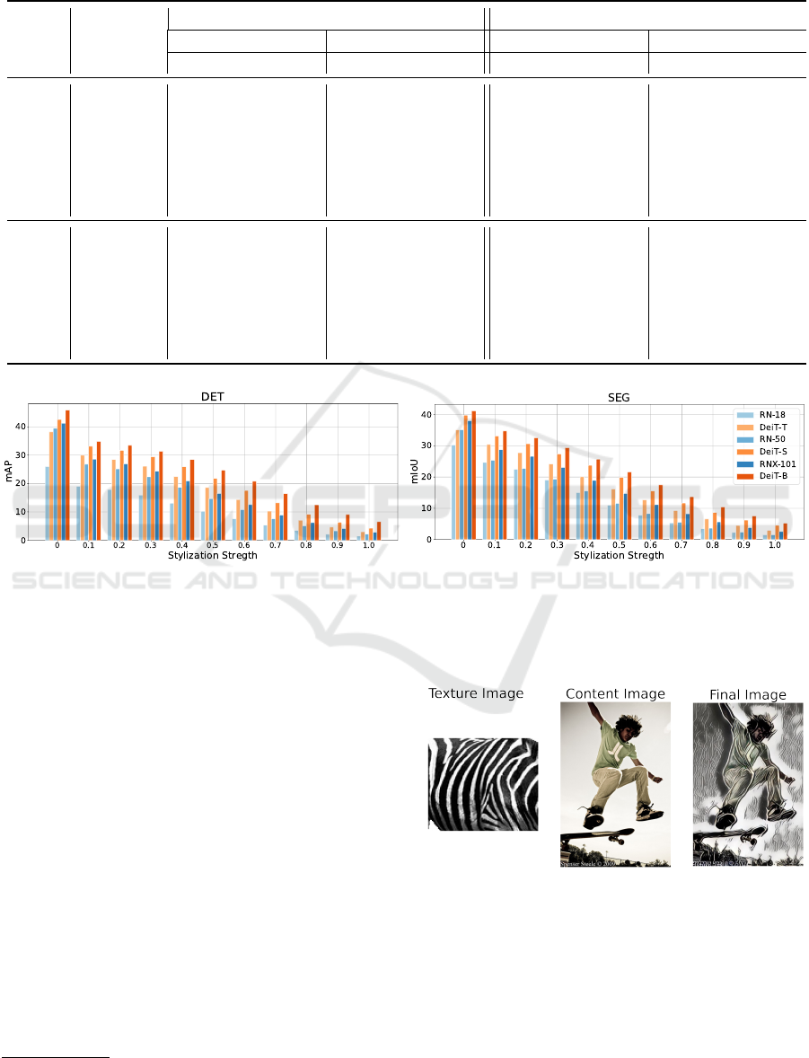
Table 5: The performance of VTs and their CNN counterparts under targeted attack when ’car’ and ’person’classes are

swapped.

‘Person’ ‘Car’

AP/IoU F1 AP/IoU F1

B A B A B A B A

DET

RN-18 0.7855 0.7707 1.0283 0.9991 0.4434 0.3916 0.5523 0.5026

DeiT-T 0.8705 0.8587 1.0766 1.0484 0.5833 0.4824 0.6915 0.6054

RN-50 0.8998 0.8831 1.0910 1.0582 0.6457 0.4030 0.7600 0.6685

DeiT-S 0.8949 0.8869 1.1048 1.0815 0.6436 0.5293 0.7525 0.6732

RNX101 0.9042 0.8822 1.0920 1.0602 0.6543 0.4026 0.7623 0.6894

DeiT-B 0.9090 0.8970 1.1238 1.0973 0.6798 0.5380 0.7983 0.7046

SEG

RN-18 0.7206 0.5709 0.8375 0.7268 0.4569 0.2468 0.6272 0.3958

DeiT-T 0.7578 0.6454 0.8621 0.7845 0.4817 0.2669 0.6499 0.4213

RN-50 0.7516 0.5721 0.8581 0.7277 0.4838 0.2438 0.6521 0.3920

DeiT-S 0.7785 0.7245 0.8753 0.8402 0.5457 0.4336 0.7060 0.6049

RNX101 0.7705 0.6383 0.8703 0.7791 0.5025 0.3061 0.6688 0.4687

DeiT-B 0.7899 0.7282 0.8826 0.8426 0.5395 0.4559 0.7008 0.6263

Figure 10: Performance comparison of VTs and their CNN counterparts on stylized validation sets with increasing stylization

strength.

APPENDIX

COCO Texture Stylization for Dense

Prediction Tasks

Here, we conduct an additional study on texture-bias

of VTs and CNNs. For this, we apply a random tex-

ture from an object to every image in the COCO vali-

dation set with increasing strength of stylization using

AdaIN-style (Huang and Belongie, 2017)

. A texture

is applied only if the source object is not present in the

target image. Figure 11 shows an example of applying

a texture of a zebra on an image. Figure 10 demon-

strates that VTs continue to rely less on texture-cues

compared to CNNs at all stylization strengths. This

is in line with our results in Section 8. The higher

performance of VTs over CNNs with increasing styl-

ization strength is also indicative of their higher ro-

https://github.com/xunhuang1995/AdaIN-style

bustness to distribution shifts.

Figure 11: Texture stylization of an image with person and

skateboard with texture of zebra, at stylization strength 0.4.

A Comprehensive Study of Vision Transformers on Dense Prediction Tasks

223