Machine Learning-based Study of Dysphonic Voices for the
Identification and Differentiation of Vocal Cord Paralysis and Vocal
Nodules
Valerio Cesarini
1a
, Carlo Robotti
2b
, Ylenia Piromalli
1c
, Francesco Mozzanica
3d
,
Antonio Schindler
4e
, Giovanni Saggio
1f
and Giovanni Costantini
1g
1
Department of Electronic Engineering, University of Rome Tor Vergata, Rome, Italy
2
Department of Otolaryngology - Head and Neck Surgery, University of Pavia, Pavia, Italy
3
Department of Clinical Sciences and Community Health, University of Milan, Milan, Italy
4
Department of Biomedical and Clinical Sciences, L. Sacco Hospital, University of Milan, Milan, Italy
Keywords: Machine Learning, Voice Analysis, Dysphonia, CFS, SVM, Biomarkers, MFCC, Energy, Shimmer, Vocal
Cords, Vocal Folds, Nodules, Paralysis.
Abstract: Dysphonia can be caused by multiple different conditions, which are often indistinguishable through
perceptual evaluation, even when undertaken by experienced clinicians. Furthermore, definitive diagnoses are
often not immediate and performed only in clinical settings through laryngoscopy, which is an invasive
procedure. This study took into account Vocal Cord Paralysis (VCP) and Vocal Nodules (VN) given their
perceptual similarity and, with the aid of euphonic control subjects, aimed to build a framework for the
identification and differentiation of the diseases. A dataset of voice recordings comprised of 87 control
subjects, 85 subjects affected by VN, and 120 subjects affected by VCP was carefully built within a controlled
clinical setting. A Machine-Learning framework was built, based on a correlation-based feature selection
bringing relevant biomarkers, followed by a ranker and a Gaussian Support Vector Machine (SVM) classifier.
The results of the classifications were promising, with the comparisons versus healthy subjects bringing
accuracies higher than 98%, while 89.21% was achieved for the differentiation. This suggests that it may be
possible to automatically identify dysphonic voices, differentiating etiologies of dysphonia. The selected
biomarkers further validate the analysis highlighting a trend of poor volume control in dysphonic subjects,
while also refining the existing literature.
1 INTRODUCTION
1.1 A Background on Dysphonia
Dysphonia can be defined as a qualitative and/or
quantitative alteration of voice production, which can
represent the result of several pathological conditions.
Approxilmately 10% of the general population may
experience dysphonia at least once in a lifetime
a
https://orcid.org/0000-0002-8305-3604
b
https://orcid.org/0000-0002-2731-9754
c
https://orcid.org/0000-0003-3780-8129
d
https://orcid.org/0000-0003-2591-4063
e
https://orcid.org/0000-0002-8767-5179
f
https://orcid.org/0000-0002-9034-9921
g
https://orcid.org/0000-0001-8675-5532
(Martins et al., 2016). Dysphonia can be associated to
different clinical conditions with different levels of
severity. For example, a breathy voice could be
related either to vocal nodules (VN) or to vocal cord
paralysis (VCP), two forms of dysphonia which are
very common among the general population
(Mozzanica et al., 2015). However, while VN
generally represent the result of vocal abuse and
misuse, VCP can be related to more threatening
Cesarini, V., Robotti, C., Piromalli, Y., Mozzanica, F., Schindler, A., Saggio, G. and Costantini, G.
Machine Learning-based Study of Dysphonic Voices for the Identification and Differentiation of Vocal Cord Paralysis and Vocal Nodules.
DOI: 10.5220/0010913800003123
In Proceedings of the 15th International Joint Conference on Biomedical Engineering Systems and Technologies (BIOSTEC 2022) - Volume 4: BIOSIGNALS, pages 265-272
ISBN: 978-989-758-552-4; ISSN: 2184-4305
Copyright
c
 2022 by SCITEPRESS – Science and Technology Publications, Lda. All rights reserved
265

conditions such as viral infections or even cancer
(Wang et al., 2020; Todisco et al., 2021). To better
assess the underlying etiologies of dysphonic
patients, diagnostic workups are conducted in clinical
environments following standardized guidelines
including objective and subjective evaluations
(Schindler et al., 2013; Mozzanica et al., 2017;
Robotti et al., 2019; Schindler et al., 2010). However,
such diagnostic procedures are usually carried out
later than the actual development of dysphonia.
Moreover, these exams are generally expensive (as
they require qualified healthcare professionals) and
potentially invasive like a laryngoscopy (Maher et al.,
2019).
1.2 State-of-the-Art for Machine
Learning-based Speech Analysis
In recent years there has been a growing interest in
the development of methods for automatic diagnosis
and screening of dysphonia only using vocal
recordings of patients. This type of diagnosis would
not only allow the detection of the pathology at an
early stage, but would also offer the chance of a
significantly cheaper and safer medical procedure.
A pre-diagnosis based on an automatic, AI-based
analysis of the speech signal has already been proven
to be feasible, predictably more reliably for
pathologies that directly affect the phonatory system,
but not strictly limited to that (Asci et al., 2021; Suppa
et al., 2021).
A review of papers on the topic published in 2019
(Sarika et al., 2019) showed that the most widely used
classification method appears to be that based on
Support Vector Machine (SVM) (Cortes and Vapnik,
1995), which is in line with the fact that it is a very
effective classifier for small datasets like the ones
encountered in the literature.
In a 2016 study (Forero et al, 2016), classification
using SVM provided better results than those based
on ANN and HMM, reaching an accuracy rate of
97.2%. However, the dataset used is rather small, and
all people with dysphonia due to nodules are female.
In a 2018 paper (Dankovičová et al., 2018), a
dataset consisting of 94 samples of objects with
dysphonia and 100 samples of healthy subjects was
used. The samples contained the vowels /a/, /e/, and
/u/, and an initial number of 1560 features (130 for
each vowel pitch), but only the vowel /a/ with
approximately 300 features, using an SVM classifier,
brought the best accuracy levels, the highest one
being 86.2% obtained with only male samples. Even
in the recent years, SVM has still proven itself as a
very accurate alternative to Deep Learning models for
reduced datasets of dysphonic voices (Costantini et
al., 2021).
Other studies report satisfactory results, but rarely
focus on the distinction between diseases in
classifying sick subjects. Our aim is to improve the
classification accuracy for the identification of
dysphonic conditions, starting from the collection of
a clean and homogeneous dataset, which will then be
processed with a problem-specific, fine-tuned
machine learning pipeline. Moreover, we also focus
on the distinction between VCP and VN as different
causes of dysphonia, and on a preliminary study on
pre- and post-treatment VCP and its effects on the
voice.
2 MATERIALS AND METHODS
2.1 Study Population
A total of 292 subjects, all over the age of 18, took
part in the study. Specifically, 120 subjects affected
by Vocal Cord Paralysis (VCP) and 85 subjects
affected by Vocal Nodules (VN) have been recruited
thanks to the collaboration with the Hospital of San
Matteo, Pavia. Of the VCP subjects, all recorded
before any treatment, 65 were female and 55 were
male, while the VN subjects counted 63 females and
20 males. 87 healthy control subjects of normal
weight, with no audible or diagnosed vocal
impairment were recruited from previous studies in
the University of Rome, Tor Vergata. They are
composed of 64 female and 23 male subjects, which
is approximately homogeneous to the distribution of
the sick subjects, especially for VN.
Healthy subjects will be referred to as “H”, pre-
treatment VCP will be “P1”, and VN will be “N”.
2.2 Voice Recording
Voice recordings have been performed in controlled
environment by trained personnel. Specifically,
hospital rooms that were as noise-free as possible
have been chosen, with each subject being alone in
the room with the recording personnel. Each subject
was asked to sit comfortably and vocalize the vowel
/a/ for at least 3 seconds without straining. The choice
of the specific vocal task was due to a compromise
between classification effectiveness (Suppa et al.,
2020), ease of recording for the subjects, and
neutrality of the larynx (Fant, 1960).
The recording hardware consisted in a Sennheiser
e835 dynamic microphone, with a cardioid polar
pattern, connected to a Zoom H4n hi-definition
BIOSIGNALS 2022 - 15th International Conference on Bio-inspired Systems and Signal Processing
266

digital recorder. Output files were mono .wav, with
16 bits of depth and a sampling frequency of 44100
Hz.
Each recording was checked on-site by the
personnel to make sure that no unexpected noises
occurred, with a particular attention to other voices.
Each sample was listened by ear by trained audio
engineers and voice experts.
2.3 Data Pre-processing
Three different binary classifications, also referred to
as comparisons, will be built from the collected
datasets. Two comparisons are focused on the
identification of a certain pathology, namely pre-
treatment VCP versus healthy subjects (referred to as
“P1 vs H”) and VN versus healthy subjects (“N vs
H”). A comparison between the two diseases is also
tackled (“P1 vs N”).
2.3.1 Audio Processing
All the audio files, which ultimately consisted of one
sample per subject in each class, were imported into
the Digital Audio Workstation REAPER (by Cockos)
for pre-processing. There, they endured a manual
segmentation to remove portions of non-spoken
signal at the beginning and at the end of the file.
Afterwards, they were normalized to 0dB peak
volume. Subsequently, a noise reduction algorithm
was applied using the “Spectral Denoise” plugin,
which is part of the iZotope® RX7 audio repair suite
(https://www.izotope.com/en/products/rx/features/sp
ectral-de-noise.html). The noise profile has been
“learnt” by the algorithm by evaluating silence-only
sections, and each file was listened to after the
processing, and verified as more intelligible than
before and without audible artifacts.
After noise reduction, each file was normalized
again and rendered in the same format as the original.
2.3.2 Feature Extraction
The normalized, noise-free audio files were then
transformed into data matrices by a feature extraction
process using OpenSMILE® by AudEERING
(Eyben et al., 2010).
It is a tool that allows for the automatic extraction
of an incredibly high amount of acoustic features,
depending on a “configuration” feature set. The one
chosen for this study is the INTERSPEECH
Computational Paralinguistic Challenge (ComParE)
2016 (Schuller et al., 2016). It extracts many
functionals of features spanning in the Energy and
Frequency domains as well as prosodic features),
Mel-frequency Cepstral Coefficients, or MFCC
(Bogert et al., 1963) and RASTA-PLP coefficients
(Hermansky and Morgan, 1994).
A total of 6373 features were extracted from each
file, and a data matrix (in .arff format) was created for
each comparison. As an example, the .arff file
necessary for the P1 vs H comparison had
120+87=207 rows, one for each subject, and 6374
columns, the last of which being the “class” label.
2.4 Machine Learning
All the learning algorithms have been applied to the
numeric data matrices extracted by OpenSMILE,
using the environment of Weka®, by the University
of Waikato (Eibe et al., 2016). As previously stated,
an automatic feature selection followed by a ranking
and manual selection of the top features precede the
SVM-based classification.
2.4.1 Feature Selection and Ranking
Data matrices first endured an automatic feature
selection procedure, in order to greatly reduce the
number of attributes in accordance with the principles
of the Curse of Dimensionality (Köppen, 2009). A
feature space of a much higher dimensionality than
the amount of labeled data will render such data as
sparse, which will drastically hinder the performances
of any statistical model. Although many “rules of
thumb” have been established, it is a currently
accepted principle to at least have less features than
the amount of data. Moreover, as stated by Zollanvari
et al. (Zollanvari et al., 2020), it is also important to
check for redundancy among the additional features
involved.
Thus, we opted to use an automatic method called
CFS – Correlation-based Feature Selection (Hall,
1999), which is based on a heuristic merit factor
which takes into account both the correlation between
a feature set and the class, and the redundancy among
features.
𝑀

=
𝑘∗𝑟






𝑘+𝑘
(
𝑘−1
)
∗𝑟





(1)
Where:
k I the number of features in the subset S
𝑟





is the average correlation between each
feature in the subset and the class.
𝑟





is the average cross-correlation between all
the features one with each other.
The optimal subset is selected with the aid of a
search method, which in our case was a Forward
Greedy Stepwise, which represented a good
Machine Learning-based Study of Dysphonic Voices for the Identification and Differentiation of Vocal Cord Paralysis and Vocal Nodules
267

compromise between performance and computational
complexity.
Throughout all of our comparisons, the CFS
retained a number of features which was not
predictable, although always smaller than 3% of the
original number. Thus, a manual selection followed
in order to furtherly reduce the features to a number
that was always consistent. The algorithm of choice
was a wrapped Linear SVM Classifier, trained on a
single feature at a time. This way, the features were
ranked and then the top 50 were manually retained.
2.4.2 Classification
Reduced data matrices were used to train a Gaussian
SVM classifier. Support Vector Machines are
statistical classifiers which aim to find the optimal
hyperplane for linear separation of the data. As
already stated, SVM classifiers are often chosen for
audio classification tasks with complex relationships
due to them being well-generalized even with small
datasets (Srivastava and Bhambhu, 2010; Costantini
et al., 2010). They are based on the non-linear
separation obtained by the “kernel trick”, based on
Mercer’s theorem. The corresponding kernel function
for a Gaussian SVM is:
𝐾
(
𝑥,𝑦
)
=𝑒

‖
𝒙
𝟏
𝒙
𝟐
‖

(2
)
For each pair of data points x
1
and x
2
.
The parameter γ represents the inverse weight of
the distance between two points: the higher it is, the
lower the importance of a single training example.
The SVM optimization is solved with the
Lagrangian Dual problem, which can also include a
regularization procedure that leads to a parameter C
(“Complexity”) penalizing classification errors,
according to the formula:
𝐶
|
𝑤
|


+
1
𝑛
max(0,1−𝑦

𝐻)



(3)
Where 𝐻=𝑤

𝑥−𝑏 represents the common
maximum margin hyperplane function, and with n
being the number of samples, x being the data vector,
𝑦

representing one of the two thresholds of the
binary classification (-1 and 1), w being the normal
vector to the hyperplane and b determining the offset.
A lower C value will result in less strict margins over
the separation plane: the parameter can be tuned to
prevent overfit.
For our specific study, the Gaussian SVM models
for each comparison have been tuned with different
values of γ and C. The classifier were calibrated,
according to Platt’s scaling method (Platt, 1999),
using a multinomial Logistic regressor. Thus,
formerly binary output predictions could be
transformed in a probability distribution over classes,
which also aided in the evaluation of the ROC curve
(Fawcett, 2006).
A 10-fold cross-validation has been employed to
evaluate the accuracy of the classifiers, by averaging
the test performances over each of the ten subsets.
Performance on each training example is evaluated
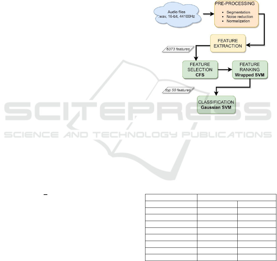
when the example is placed in the test subset. Figure
1 shows the steps of the whole pipeline.
Figure 1: Flowchart for the machine learning-based voice
analysis: from audio files to classification models.
3 RESULTS
The confusion matrices for each comparison are
presented in the following Table.
Table 1: Confusion matrices.
True Class
Classified as: P1 H
P1 119 1
H1 86
N H
N 83 1
H2 85
P1 N
P1 108 12
N 10 74
Classification accuracy percentages (abbreviated
as ACC) are displayed in Table 2 along with other
useful performance indicators. Specifically,
Sensitivity (Sens) and Specificity (Spec) are reported
along with the False Positive Rate (FPR). Sens and
BIOSIGNALS 2022 - 15th International Conference on Bio-inspired Systems and Signal Processing
268

Spec represent the True Positive Rate and the True
Negative Rate respectively, and can be calculated as
such:
𝑆𝑒𝑛𝑠 =
𝑇𝑃
𝑃𝑜𝑠
(4
)
𝑆𝑝𝑒𝑐 =
𝑇𝑁
𝑁𝑒𝑔
(5
)
𝐹𝑃𝑅 =
𝐹𝑃
𝑁𝑒𝑔
=1−𝑆𝑝𝑒𝑐
(6
)
Where TP are the True Positives, TN the True
Negatives, FP the False Positives (negative subjects
classified as positive), Pos represents all the positive
subjects (TP+False negatives) and Neg all the
negatives (TN+FP). For each of our comparisons, the
first class in the order they appear in Table 1 is
considered as positive. Control subjects are always
negative, and, for the P1 vs N comparison, N are
considered as negative.
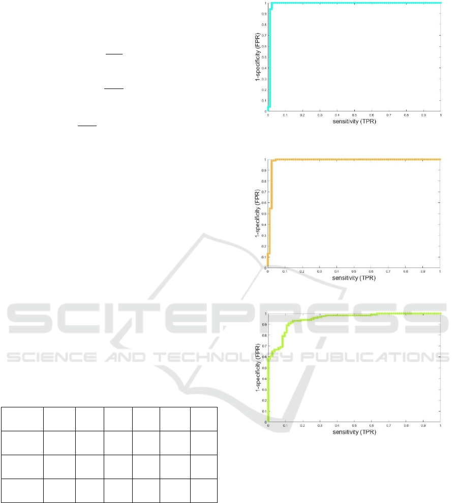
ROC curves have also been evaluated for each
classifier and are displayed in Figures 2, 3 and 4. The
area under the curve, or AUC, is reported in Table 2,
as well as the Cut-off point (CO) of each ROC curve.
Note that the AUC is generally considered as a more
general and reliable indicator for the performances of
a classifier, since it is an aggregate measure of
performance across all possible classification
thresholds. “Comp.” in the first column refers to
which comparison is being considered.
Table 2: Classification Performances.
Comp. ACC
%
Sens Spec FPR AUC CO
P1 vs H
99.03 0.99 0.99 0.01 0.99 1.00
N vs H
98.24 0.99 0.98 0.02 0.98 0.99
P1 vs N
89.21 0.9 0.88 0.12 0.95 0.91
3.1 Acoustic Features
The top ranked features, in the number of 50, are the
data on which the classifiers have been trained. Since
the very features can be fairly complex in terms of
descriptors. Considering that the most important
information is represented by the main trends in the
domains, a summary of the more prevalent acoustic
domains for each comparison is presented in Table 3.
Figure 2: ROC curve for the P1 vs H comparison.
Figure 3: ROC curve for the N vs H comparison.
Figure 4: ROC curve for the P1 vs N comparison.
Additionally, the top 5 features are presented, from
first to last, in the far-right column.
The abbreviation “std. dev” means Standard
Deviation, and “min” means Minimum. Loudness
refers to the Spectral Loudness Summation as a
weighted sum of the auditory spectrum (Anweiler and
Verhey, 2006). MFCC refers to Mel-Frequency
Cepstral Coefficients, which result from a discrete
cosine transform of the logarithmic mel-spectrum,
and identify a “frequency of frequency” useful to
describe pitch. A similar role is held by RASTA,
which refers to a RASTA-style bandpass filtering
applied to the log spectrum domain, and then applied
to a PLP (Perceptual Linear Predictive) processing
which involve the calculation of an all-pole model in
Machine Learning-based Study of Dysphonic Voices for the Identification and Differentiation of Vocal Cord Paralysis and Vocal Nodules
269

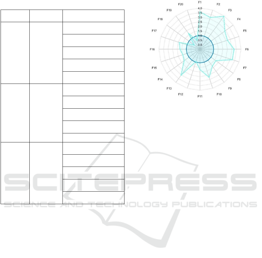
Table 3: Trends in top ranked features.
Comp. Main
Domains
Top 5 Features
P1 vs H Energy,
Loudness,
MFCC
RMS Energy (delta),
p
osition of the mean
Loudness (delta), inter-
quartile range 1-2
RMS Energy (delta), 1-
p
ercentile
Loudness (delta), inter-
q
uartile ran
g
e 1-3
RMS Energy (delta),
ran
g
e
N vs H Energy,
Spectral
Variance,
Loudness
RMS Energy (delta), Root
quadratic mean
Spectral Slope (delta),
p
osition of the mean
RMS Energy (delta), 1-
p
ercentile
Spectral Slope (delta), 99-
p
ercentile
RMS Energy, range
P1 vs N MFCC,
RASTA,
Energy
2nd MFCC, mean of
risin
g
slo
p
e
RASTA Window 1, 1-
p
ercentile
RASTA Window 0, 1-
p
ercentile
RMS Energy (delta),
Relative min ran
g
e
RASTA-style Loudness,
1-
p
ercentile
the transformed domain, followed by the calculation
of MFCC. So, a RASTA-style Loudness as it appears
in the 5
th
place for the P1 vs N comparison, is based
on a summation over a RASTA-filtered spectrum.
The Spectral Variance is used as an “umbrella term”
for features generally related to variations in the
spectrum. Includes Slope, Kurtosis, Skewness, Flux,
Harmonicity.
As an additional tool for visualizing the relative
value and the discrimination power of the selected
features, a sample radar plot for the first 20 features
is displayed in Figure 5. The reduced number of
features is due to visualization needs. The plots are
made by averaging each feature over all the instances
(subjects) and normalizing it with respect to the
“negative” class, which is always the second
according to the order found in Table 1. Each point in
the plot represents one feature, and two curves are
thus realized, the negative class always resulting in a
unit circle since it’s normalized by itself. Note that the
classifier performances are based on more
information than just the mean of the first 20 features.
Figure 5: Radar plot for the P1 vs H comparison. The darker
unit circle refers to the normalized H class.
4 DISCUSSION
Accuracies higher than 98% have been obtained for
the comparisons of dysphonic subjects versus
healthy-voiced subjects. This is quite promising
because it shows that an automatic distinction can
indeed be performed with the aid of the right features
and machine learning pipeline. On the other hand, the
lower accuracy for the P1 vs N comparison also
appears reasonable, as distinguishing between a
healthy and dysphonic voice is an easier task even in
phoniatric examinations. Specific attention has been
used in the recording environment and audio
segmentation, and specific feature selection
algorithms which we already tested extensively have
been employed in place of standardized subsets which
can be found in the literature (Saggio and Costantini,
2020). Although bias due to heterogeneity in the
subjects’ demographics is indeed possible, the
features were confronted with those typical of other
effects affecting the voice, like ageing or gender (Asci
et al., 2020).
The chosen classifier, namely a Gaussian SVM
with a logistic calibrator, has been selected basing on
the state-of-the-art, on previous experiments and on
the principle that it’s a very effective classifier for
reduced datasets. High AUC values show that the
models are indeed effective on the training set for
many threshold values.
From the observation of the features distribution
between classes, a general trend appears for sick
subjects with respect to non-dysphonic subjects. Both
P1 and N classes show a significantly higher variance
in RMS Energy, which could be consistent with a
“stale” quality of the voice and, especially, with a
BIOSIGNALS 2022 - 15th International Conference on Bio-inspired Systems and Signal Processing
270

certain lack of volume control that sick subjects may
experience. Thus, there is indeed a similarity in the
features that distinguish between VCP and healthy
subjects, and VN and healthy subjects. The latter
comparison appears to rely more on spectral
characteristics.
In fact, the differentiation of the two diseases does
not rely on the Energy domain, but it’s shown as
feasible basing mainly on RASTA-PLP filtering. This
is in line with some of our studies which show how
RASTA is a powerful tool for the identification of
complex characteristics in the voice (Cesarini et al.,
2021).
5 CONCLUSIONS
After building a polished dataset, a traditional
pipeline-based machine learning framework has been
established for the detection of VCP and VN versus
healthy control subjects, and the differentiation
between the two diseases. A feature selection helped
identify acoustic features as specific biomarkers for
each comparison, which were then used for the
training of SVM models. The classification results
show a very high accuracy in distinguishing patients
from healthy subjects, in fact the highest among
similar studies. A lower but still significant accuracy
was obtained for the differentiation between diseases.
This is in line with the complexity of the problem
when faced on a phoniatric point of view, and also
proves that a distinction can be made even when the
effects on the voice aren’t evident by ear. Energy-
level characteristics are used for the distinction of a
dysphonic voice from a healthy one, suggesting a lack
of voice volume control in dysphonic subjects, while
RASTA and Cepstral domains are relevant for the
differentiation of the diseases.
The whole framework would benefit from the
collection of more data, which is foreseeable since the
environment and collaborations are ongoing.
This kind of vocal analysis can be of great help in
the diagnostics of dysphonic diseases, especially
since currently used methods are often slow and
invasive. The automatic voice analysis as well as the
observation of acoustic features can also aid
phoniatric examinations, replacing or supporting
evaluations made by-ear. In this perspective, a more
thorough study of the selected features, possibly
refined by a bigger dataset, will help identifying the
best possible subsets, specific to each disease or
comparison. Moreover, automatic tools can be built
for on-site classification, helping in preliminarily
identifying different dysphonic conditions. Although
automatic voice analysis per se cannot substitute a
medical diagnosis, the possibilities offered by this
technology appear to be very wide and promising.
ACKNOWLEDGEMENTS
This study was supported in part by Voicewise S.r.l.,
and thanks to the precious collaborations of the
Hospital of San Matteo, Pavia, and of the University
of Rome Tor Vergata.
REFERENCES
Anweiler, A., Jesko L.V. (2006). Spectral loudness
summation for short and long signals as a function of
level. In: Journal of Voice, The Journal of the
Acoustical Society of America 119, 2919-2928 (2006)
Asci , F., Costantini, G., Saggio, G., Suppa, A. (2021).
Fostering Voice Objective Analysis in Patients with
Movement Disorders. In: Movement Disorders, vol. 36,
ISSN: 0885-3185
Asci, F., Costantini, G., Di Leo, P., Zampogna, A.,
Ruoppolo, G., Berardelli, A., Saggio, G., & Suppa, A.
(2020). Machine-Learning Analysis of Voice Samples
Recorded through Smartphones: The Combined Effect
of Ageing and Gender. In: Sensors (Basel,
Switzerland), 20(18), 5022.
Bogert, B.P., Healy, M.J.R., Tukey J.W. (1963). The
Quefrency Alanysis [sic] of Time Series for Echoes:
Cepstrum, Pseudo Autocovariance, Cross-Cepstrum
and Saphe Cracking, Proceedings of the Symposium on
Time Series Analysis (M. Rosenblatt, Ed) Chapter 15,
209-243. New York: Wiley.
Cesarini, V., Casiddu, N., Porfirione, C., Massazza, G.,
Saggio, G., Costantini, G. (2021). A Machine Learning-
Based Voice Analysis for the Detection of Dysphagia
Biomarkers, In: 2021 IEEE MetroInd4.0&IoT, 2021.
Cortes, C.; Vapnik, V.N. (1995). "Support-vector
networks" (PDF). In: Machine Learning.
Costantini, G., Casali, D., Todisco, M. (2010), “An SVM
based classification method for EEG signals”,
Proceedings of the 14th WSEAS international
conference on Circuits, 107–109.
Costantini, G., Di Leo, P., Asci, F., Zarezadeh, Z., Marsili,
L., Errico, V., Suppa, A., Saggio, G. (2021). Machine
learning based voice analysis in spasmodic dysphonia:
An investigation of most relevant features from specific
vocal tasks. In: BIOSIGNALS 2021. Vienna, Austria,
2021
Dankovičová, Z.; Sovák, D.; Drotár, P.; Vokorokos, L.
(2018). Machine Learning Approach to Dysphonia
Detection. Appl. Sci. 2018, 8, 1927.
Eibe, F., Hall, M. and Witten, I. (2016). The WEKA
Workbench. Online Appendix for Data Mining:
Practical Machine Learning Tools and Techniques,
Morgan Kaufmann, Fourth Edition, 2016.
Machine Learning-based Study of Dysphonic Voices for the Identification and Differentiation of Vocal Cord Paralysis and Vocal Nodules
271

Eyben, F., Wöllmer, M., Björn Schuller, M. (2010).
openSMILE - The Munich Versatile and Fast Open-
Source Audio Feature Extractor, Proc. ACM
Multimedia (MM), ACM, Florence, Italy, ISBN 978-1-
60558-933-6, pp. 1459-1462, 25.-29.10.2010.
Fant, G. (1960). Acoustic Theory of Speech Production.
The Hague: Mouton.
Fawcett, Tom (2006). An Introduction to ROC Analysis In:
Pattern Recognition Letters. 27 (8): 861–874.
Forero M, L. A., Kohler, M., Vellasco, M. M., & Cataldo,
E. (2016). Analysis and Classification of Voice
Pathologies Using Glottal Signal Parameters. Journal
of voice: official journal of the Voice Foundation,
30(5), 549–556.
Hall, Mark A. (1999). Correlation-based Feature Selection
for Machine Learning. University of Waikato,
Department of Computer Science, Hamilton, NZ.
Hermansky, Hynek & Morgan, Nathaniel. (1994). RASTA
processing of speech. In: IEEE Transactions on Speech
and Audio Processing.
Köppen, Mario. (2009). The Curse of Dimensionality.
10.1007/978-0-387-39940-9_133.
Maher, D. I., Goare, S., Forrest, E., Grodski, S., Serpell, J.
W., & Lee, J. C. (2019). Routine Preoperative
Laryngoscopy for Thyroid Surgery Is Not Necessary
Without Risk Factors. Thyroid: official journal of the
American Thyroid Association, 29(11), 1646–1652.
Martins RH, do Amaral HA, Tavares EL, Martins MG,
Gonçalves TM, Dias NH. Voice Disorders: Etiology
and Diagnosis. J Voice. 2016
Moore, R., Lopes, J. (1999). Paper templates. In:
TEMPLATE’06, 1st International Conference on
Template Production. SCITEPRESS.
Mozzanica F, Ginocchio D, Barillari R, et al. (2016).
Prevalence and Voice Characteristics of Laryngeal
Pathology in an Italian Voice Therapy-seeking
Population. Journal of Voice. 2016 Nov;30(6):774.e13-
774.e21.
Platt, John (1999). "Probabilistic outputs for support vector
machines and comparisons to regularized likelihood
methods". In: Advances in Large Margin Classifiers. 10
(3): 61–74.
Saggio G, Costantini G (2020). Worldwide Healthy Adult
Voice Baseline Parameters: A Comprehensive Review.
Journal of Voice, ISSN: 0892- 1997
Sarika, H., Surendra, S., Smitha, R., Thejaswi, D.. (2019).
A Survey on Machine Learning Approaches for
Automatic Detection of Voice Disorders, In: Journal of
voice: official journal of the Voice Foundation.
Schindler, A., Mozzanica, F., Maruzzi, P., Atac, M., De
Cristofaro, V., & Ottaviani, F. (2013).
Multidimensional assessment of vocal changes in
benign vocal fold lesions after voice therapy. Auris,
nasus, larynx, 40(3), 291–297.
Schindler, A., Ottaviani, F., Mozzanica, F., Bachmann, C.,
Favero, E., Schettino, I., & Ruoppolo, G. (2010). Cross-
cultural adaptation and validation of the Voice
Handicap Index into Italian. Journal of voice: official
journal of the Voice Foundation, 24(6), 708–714.
Schuller, B., Steidl, S., Batliner, A.,Hirschberg, J.,
Burgoon, J., Baird, A.,Elkins, A.,Zhang, Y., Coutinho,
E., Evanini, K. (2016). The INTERSPEECH 2016
Computational Paralinguistics Challenge: Deception,
Sincerity and Native Language. 2001-2005. In:
INTERSPEECH, 10.21437/Interspeech.2016-129.
Smith, J. (1998). The book, The publishing company.
London, 2
nd
edition.
Srivastava, Durgesh & Bhambhu, Lekha. (2010). Data
classification using support vector machine. In: Journal
of Theoretical and Applied Information Technology.
12. 1-7.
Suppa, A., Asci ,F., Saggio ,G., Di Leo, P., Zarezadeh, Z.,
Ferrazzano, G., Ruoppolo, G., Berardelli, A.,
Costantini, G. (2021). Voice Analysis with Machine
Learning: One Step Closer to an Objective Diagnosis of
Essential Tremor. In: Movement Disorders.
Suppa, A., Asci, F., Saggio, G., Marsili, L., Casali, D.,
Zarezadeh, Z., Ruoppolo, G., Berardelli, A., Costantini,
G. (2020). Voice analysis in adductor spasmodic
dysphonia: Objective diagnosis and response to
botulinum toxin. In: Parkinsonism and Related
Disorders, ISSN: 1353-8020
Todisco, M., Alfonsi, E., Arceri, S., et al. (2021). Isolated
bulbar palsy after SARS-CoV-2 infection. Lancet
Neurology 2021 Mar;20(3):169-170.
Wang, H.W., Lu, C.C., Chao, P.Z., Lee , F.P. (2020).
Causes of Vocal Fold Paralysis. Ear Nose Throat J.
2020 Oct 22:145561320965212. doi: 10.1177/
0145561320965212. Epub ahead of print.
Zollanvari, A., James, A.P. & Sameni, R. (2020). A
Theoretical Analysis of the Peaking Phenomenon in
Classification. J Classif 37, 421–434.
BIOSIGNALS 2022 - 15th International Conference on Bio-inspired Systems and Signal Processing
272