Combining YOLO and Deep Reinforcement Learning for
Autonomous Driving in Public Roadworks Scenarios
Nuno Andrade
1
, Tiago Ribeiro
1a
, Joana Coelho
2a
, Gil Lopes
3c
and A. Fernando Ribeiro
1d
1
Department of Industrial Electronics, ALGORITMI CENTER, University of Minho, Guimarães, Portugal
2
Department of Mechanical Engineering, University of Minho, Guimarães, Portugal
3
Department of Communication Sciences and Information Technologies, University of Maia, Maia, Portugal
Keywords: Deep Learning, YOLO, Reinforcement Learning, Deep Deterministic Policy Gradient, Autonomous Driving,
Public Roadworks.
Abstract: Autonomous driving is emerging as a useful practical application of Artificial Intelligence (AI) algorithms
regarding both supervised learning and reinforcement learning methods. AI is a well-known solution for some
autonomous driving problems but it is not yet established and fully researched for facing real world problems
regarding specific situations human drivers face every day, such as temporary roadworks and temporary signs.
This is the core motivation for the proposed framework in this project. YOLOv3-tiny is used for detecting
roadworks signs in the path traveled by the vehicle. Deep Deterministic Policy Gradient (DDPG) is used for
controlling the behavior of the vehicle when overtaking the working zones. Security and safety of the
passengers and the surrounding environment are the main concern taken into account. YOLOv3-tiny achieved
an 94.8% mAP and proved to be reliable in real-world applications. DDPG made the vehicle behave with
success more than 50% of the episodes when testing, although still needs some improvements to be
transported to the real-world for secure and safe driving.
1 INTRODUCTION
In recent years, AI is becoming highly researched
regarding autonomous driving (Arcos-García et al.,
2018b; Chun et al., 2019). Researchers are constantly
studying ways to make autonomous vehicles reliable
in the context of real-world applications (Kaplan
Berkaya et al., 2016; Lim et al., 2017). In some
situations, it might be required to have temporary
road signs which by default can alter the previously
standard regulation. The new temporary road signs
can overlap the normal road rules and therefore the
vehicles must ignore the standard rules and follow the
specific ones. Recently, some studies have been
conducted in regard of this subject, namely in
Formula Student competition (Svecovs &
Hörnschemeyer, 2020), however, there is still a gap
in scientific research (Liu et al., 2021). The majority
of the solutions do not necessarily use supervised
a
https://orcid.org/0000-0002-5909-0827
b
https://orcid.org/0000-0002-5992-975X
c
https://orcid.org/0000-0002-9475-9020
d
https://orcid.org/0000-0002-6438-1223
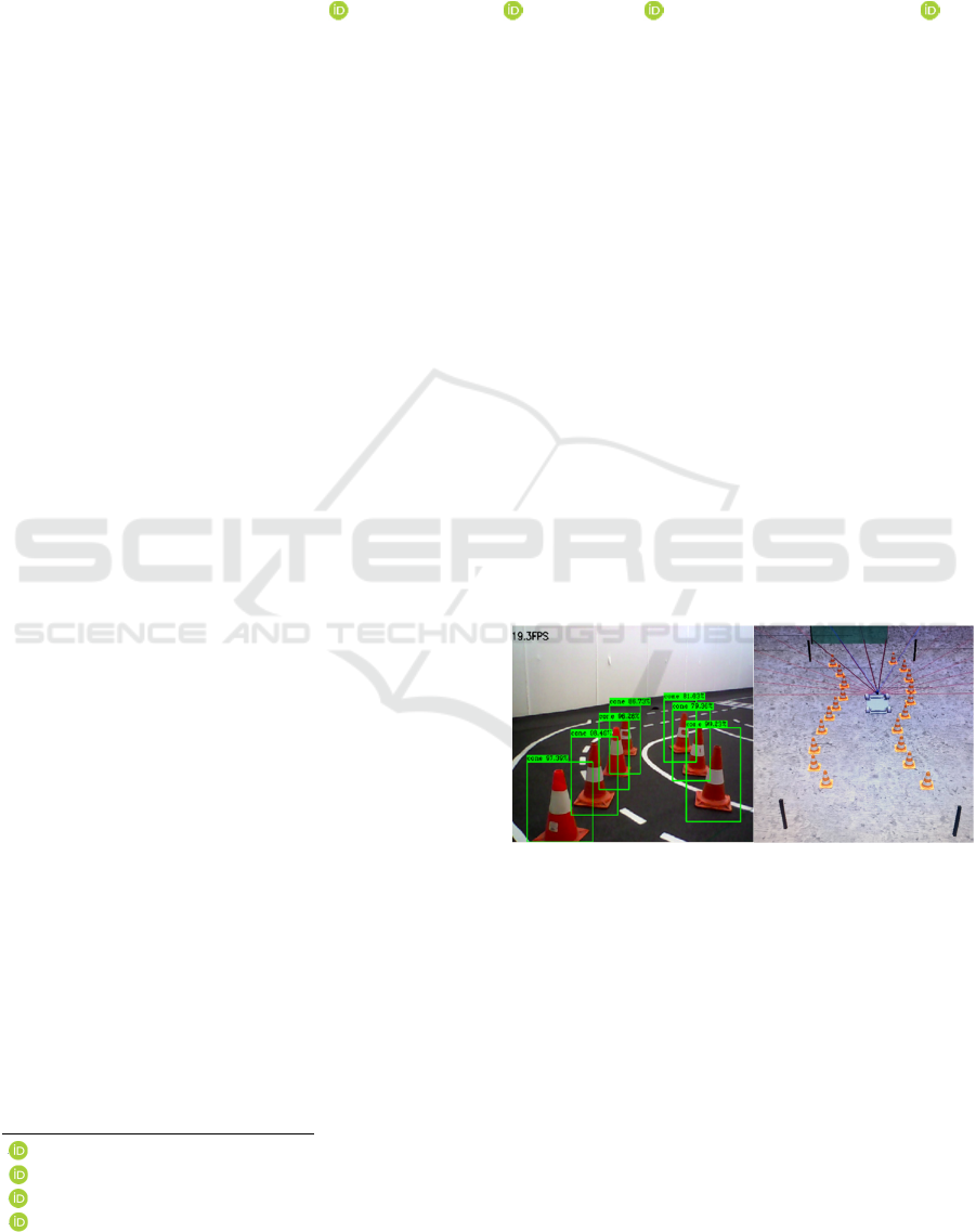
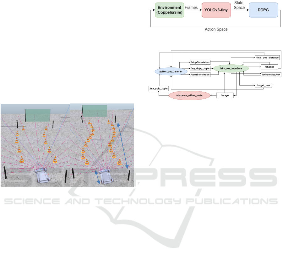
Figure 1: Detection of the roadworks signs and vehicle’s
movement control.
learning and reinforcement learning combined. This
project combines YOLOv3-tiny and DDPG for
solving roadworks signs detection and the vehicle’s
behavior control in those real-world situations. Both
use neural networks, although in different contexts.
Figure 1 presents the detection module and the
planning of motion in real-time.
Andrade, N., Ribeiro, T., Coelho, J., Lopes, G. and Ribeiro, A.
Combining YOLO and Deep Reinforcement Learning for Autonomous Driving in Public Roadworks Scenarios.
DOI: 10.5220/0010913600003116
In Proceedings of the 14th International Conference on Agents and Artificial Intelligence (ICAART 2022) - Volume 3, pages 793-800
ISBN: 978-989-758-547-0; ISSN: 2184-433X
Copyright
c
2022 by SCITEPRESS – Science and Technology Publications, Lda. All rights reserved
793
The system receives sensorial information
through a strategic camera and 16 sensors placed at
the front of the vehicle. This solution does not require
hard transformations to the chassis used in common
vehicles, making it more suitable for manufacturers
to apply the concepts.
Usually, authors present two main approaches for
autonomous driving problems which are end-to-end
and modular (T. Ribeiro et al., 2019; Huang & Chen,
2020; Yurtsever et al., 2020). This project follows the
second approach in order to simplify the complexity
of the problem. In case of system fail or upgrade
system components, maintenance becomes a simpler
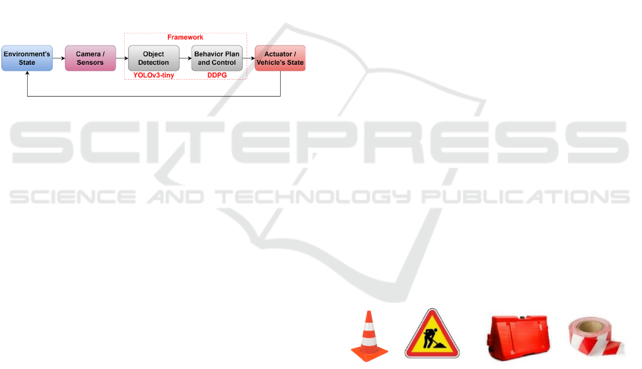
task. The main tasks that the framework is supposed
to handle are: a) to process the detection of temporary
roadworks signs (object detection); b) to process the
data from the previous task commanding the vehicle
(Behavior Plan and Control) to act (Actuator) the
optimal way for the current state of the environment.
Figure 2 portrays the proposed framework.
Figure 2: Project modular-based approach and
implementation of the autonomous driving framework.
YOLOv3-tiny can detect multiple objects from
different classes at high frame rates. This is crucial for
maintaining the security and safety, since good
reflexes are expected from a human driver as well.
The vehicle also needs to be able to perform and
behave with efficiency and precaution. Many pieces
of research use deep reinforcement learning to
accomplish that performance (Sallab et al., 2017;
Kiran et al., 2021) and so DDPG is chosen for this
project. DDPG is suitable for real-world complex
robotic tasks and it uses neural networks to learn from
the environment and deploy the best vehicle behavior
it can achieve. For that, it chooses the action that leads
to the best reward achievable. This paper is composed
by a brief introduction of YOLOv3-tiny, the dataset
on which it was trained, a summary of DDPG and its
configuration, the simulation environment used, how
the communication was made between the framework
modules as well as the final results and the
correspondent conclusions.
2 YOLOv3-tiny
YOLOv3-tiny (Adarsh et al., 2020) is an one-stage
object detection algorithm proposed by J.Redmon
(Redmon & Farhadi, 2018) which focus on high
frame rates, taking advantage of YOLOv3 best
features. The architecture of YOLOv3-tiny is mainly
composed by convolution layers followed by max-
pooling layers to perform feature extraction from the
input images divided into SxS grid cells. YOLOv3-
tiny is fast because it operates only at two different
map scales which are 13x13 and 26x26, for 416x416
input images. It is able to detect medium-large objects
since for those scales small objects remain
undetectable.
For predicting the bounding boxes, YOLOv3-tiny
uses the same concepts of YOLOv3. It relies on the
use of anchor boxes to indicate the algorithm possible
locations of the objects that it is trying to detect. The
anchor boxes can be changed according to the dataset
in which YOLOv3-tiny is trained. The predicted
bounding box coordinates are calculated by the offset
between the predicted bounding box and the anchor
boxes. Finally, a threshold is used as a filter to
eliminate the bounding boxes that have low accuracy
and therefore are not useful to classify objects. The
remaining bounding boxes are excluded using Non-
Maximum Suppresion (NMS). It uses Intersection
over Union (IoU) for evaluating how coincident the
predicted bounding boxes are to the ground truth
bounding boxes and remove the least coincident ones.
3 DATASET OF YOLOv3
The dataset used for training YOLOv3-tiny contains
1252 photos with four objects randomly applied: 1)
Street cone; 2) Roadworks sign; 3) Road Separator;
4) Red and White Tape. These objects are presented
in figure 3.
Figure 3: The four objects used in the dataset.
The datasets found for these objects are not many,
these also lack in quality and have poor
diversification. To make up for these flaws, a new
entire dataset was built from scratch and every image
was tweaked to be different from the one behind and
after it. The goal was to avoid unnecessary
correlations between the images. Every image differs
in number of signs, different types of signs, hue,
saturation, brightness, shadows, object size,
perspective, contrast, color temperature, blur, noise,
ICAART 2022 - 14th International Conference on Agents and Artificial Intelligence
794
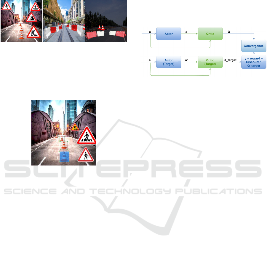
distortion and light conditions. Figure 4 shows some
examples.
Figure 4: Examples of images picked directly from the
dataset.
This extra work resulted in gradual improvements
in the algorithm response as it is described in the
Results section. The LabelImage Tool was used to
label the entire dataset images. Figure 5 shows how
the images were labeled.
Figure 5: Signs surrounded by bounding boxes manually
applied, also known as labelling.
Some signs were intentionally positioned in the
image to teach the algorithm to ignore them, so they
are not labeled. One of YOLOv3-tiny advantages is
that it does not require a large dataset to show good
results. Approximately 2000 images were used to
make the algorithm reach an mAP above 90%.
4 DEEP DETERMINISTIC
POLICY GRADIENT (DDPG)
DDPG is the brain behind the vehicle actuator. It is a
model-free, off-policy and actor-critic based model
that uses a deterministic policy and deep neural
networks to improve the actions of the vehicle in a
way that leads to obtain the maximum rewards that it
can achieve in a certain environment. The authors
(Lillicrap et al., 2016) presented it as a solution to
Deep Q-Networks limitations regarding the
continuous domains. The main characteristics of this
algorithm makes it a good fit in the autonomous
driving field where the environments typically are
continuous, complex and there is no environment
model previously known (Wang et al., 2018). DDPG
relies only in experience and trial-and-error. At first,
the trial-and-error based training can be exhaustive
but once the algorithm starts learning it results in very
robust solutions. Figure 6 represents the DDPG
architecture.
Figure 6: DDPG Structure.
Actor-Critic based methods like DDPG use neural
networks so the policy can predict actions, called a,
for the incoming states, called s, with the main goal
of obtaining the optimal Q pair. Since there is no
reference or labeled dataset that indicates what is the
optimal pair, DDPG uses target networks to estimate
the optimal value for the next state, called Q_target.
It is possible to find what is the optimal Q, called y
(in figure 6). Q must converge to y and the target
networks cannot be regularly updated like the original
ones otherwise Q_target would change a lot on each
step and thus it would be difficult to converge Q. So,
the target network is fed with weights that are softly
updated.
The optimal behavior for the vehicle is established
by a reward system so that in exploitation, the policy
learns what are the actions highly rewarded according
to a certain state. The reward system created in this
work is expressed as:
reward = A * speed
instant
– B * distance
finish_line
– C *
∆
angle
direction
– D *step
(1)
Where speed
instant
is the current speed of the
vehicle, the distance
finish_line
is the distance between
the vehicle and the finish line, the ∆
direction
is the
vehicle’s changing of direction and the step is a
counter in every episode to ensure the vehicle
executes the path in the shortest time possible. A, B,
C and D are coefficients used to adjust the impact of
each variable of the reward function, depending on
the vehicle’s behavior.
Regarding the state space and action space of
DDPG, they are respectively the following:
S = {intersection
matrix
, distance
finish_line
}
(2)
A = {steering
applied
, speed
applied
}
(3)
Combining YOLO and Deep Reinforcement Learning for Autonomous Driving in Public Roadworks Scenarios
795
In the state space, the intersection
matrix
is a matrix
of 16x3 dimensions and is the result of the visual
processing applied to every frame of the simulation.
The distance
finish_line
is the same variable as the one in
the reward system. In the action space, the
steering
applied
and the speed
applied
are the steering and
speed commanded to the actuator, respectively.
The origin of the intersection
matrix
is shown in
figure 7. One can see a set of 16 line segments rooted
in a single point in the lowest center of the frame.
These are separated by an angle of 12 degrees in the
interval of 180 degrees.
Figure 7: Image processing applied in a frame.
The line segments serve as a simpler orientation
for DDPG to know where the obstacles are and react
quickly to avoid them, rather than computing the local
coordinates of the objects detected. For instance,
every time a cone intersects one of the 16 line
segments, the line segment turns red and a flag is
generated and stored in the first column of the matrix
(and in the line correspondent to the line segment
number) that will be fed into the neural network. In
the second column of the matrix, it is stored a value
between 0 and 1, which corresponds to the distance
of the intercepted cone to the vehicle, calculated by
using visual processing techniques. In case more than
one cone intersects the same line segment, only the
nearest one is considered. On the other hand, if a line
segment is not intercepted by any cone, the distance
value is set to 1. To contextualize, 1 is estipulated as
an unreachable distance so it is the distance value
assigned to the cases where the line segments are not
intercepted.
The third column considers what line segments
are intercepted by the target. To achieve that,
proximity sensors were introduced (figure 8).
Figure 8: Sensors placed in the vehicle. The line of the
sensors blink yellow when intercepting the target.
The sensors were disposed following the same
orientation of the 16 line segments displayed in the
frame. This allows to map the target flags with the
correspondent line segments in the matrix. The goal
of the sensors is to give the vehicle an insight into the
position of the target, mainly in accentuated curves,
where the camera cannot see the target. Besides the
target, all other objects remain invisible for the
sensors. Table 1 shows a resulting matrix example.
Table 1: Matrix generated by the processing applied to the
figure 7 captured frame.
Line
Number
Intersection Distance
(%)
Target
1 0 1.0 0
2 0 1.0 0
3 0 1.0 0
4 0 1.0 0
5 1 0.39 0
6 1 0.53 0
7 1 0.63 0
8 0 1.0 1
9 1 0.73 1
10 1 0.725 0
11 0 1.0 0
12 1 0.4 0
13 0 1.0 0
14 0 1.0 0
15 0 1.0 0
16 0 1.0 0
To analyze table 1, one must look at figure 7 and
count the line number from the right to the left (the
same orientation of the unit circle). In this work,
proximity sensors are used for detecting the target,
although in real world the target coordinates are
known.
ICAART 2022 - 14th International Conference on Agents and Artificial Intelligence
796
5 SIMULATION ENVIRONMENT
CoppeliaSim was the simulator chosen to build the
environment and test the algorithms. The virtual
space contains a car and two arrays of cones. In
addition, there is a starting line and a finish line. The
vehicle length is approximately 0.8 meters and the
distance of the track is about 5 meters. These
dimensions were chosen according to the scenarios
proposed by Festival Nacional de Robótica
competition (Portuguese Robotic Festival). Figure 9
shows two of the main paths used to train and test the
system. The goal of the agent was to command
actions to the vehicle through the analysis of the
scenario using the camera which is strategically
placed in the top center of the vehicle’s roof.
Figure 9: Environment used for training and testing the
vehicle. A curve path and a double curve path, respectively.
When the DDPG episode starts, it automatically
starts the environment and sends the variables to the
car to start moving. The episode ends when the
vehicle reaches the finish line, is outside the limits,
stops or crashes against a cone. To improve the
algorithm training and reliability, in every episode the
vehicle starts at a random orientation, between ± 30
degrees. This ensures that the algorithm does not
overfit or becomes partially biased by its initial
position.
6 SYSTEM COMMUNICATION
Communication between the modules in the
simulation environment is achieved by using the
Robotic Operating System (ROS). In figure 10, two
diagrams represent the messages that are sent or
received along with the corresponding publisher or
subscriber nodes, respectively. The diagram a) is a
brief representation to better interpret what
information is required to be sent and received. It is a
simple representation of the diagram b) adapted from
a ROS tool, rqt_graph.
a)
b)
Figure 10: ROS structure.
Following the bottom diagram, the topic “/image”
receives the frames captured by the vehicle’s camera
and sends it to the YOLOv3-tiny node (called
“distance_offset_node”). After YOLOv3-tiny
processes that frame, it sends the matrix with the
intersected lines to the DDPG node (called
“talker_and_listener”) through the “/my_yolo_topic”
topic. After DDPG obtains the relevant information
regarding the environment’s state space, it sends the
proper action space to CoppeliaSim through
“/my_ddpg_topic”, receiving it in the
“sim_ros_interface” node. This node is also
responsible to send three important variables for
DDPG processing using three topics: 1) “/chatter”
sends the instant speed; 2) “/final_pos_distance"
sends the distance to the final line; 3) “/target_pos”
sends the sensors flags triggered when encountered
the target. ROS is operating at 5 Hz for all modules
due to YOLOv3-tiny processing time.
7 RESULTS
The system was implemented, trained and tested in an
Asus laptop with Intel Quad-Core i5, 2.30GHz,
Nvidia Geforce 940M GPU using Ubuntu 18.04.5
LTS 64-bit as the Operating System. For the
programming environment the main language was
Python alongside libraries such as OpenCV,
Tensorflow and Keras. YOLOv3-tiny was trained in
Google Colab due to its computational power. The
following list shows the training hyperparameters for
YOLOv3-tiny along with the chosen values: Number
of epochs = 100; Dataset split = 80% training / 20%
0.8m
5m
Combining YOLO and Deep Reinforcement Learning for Autonomous Driving in Public Roadworks Scenarios
797
testing; Learning Rate = 0.0001; Batch Size = 4;
Kernel Regularizer = 0.001; Leaky ReLU (alpha) =
0.3; Data Augmentation = On ; Input image resolution
= 416x416; IoU loss threshold = 0.5; Non-Maximum
Suppression (sigma) = 0.3; Score threshold = 0.3; IoU
threshold = 0.45.
Anchors = [[[10, 14], [23, 27], [37, 58]],
[[81, 82], [135, 169], [344, 319]],
[[0, 0], [0, 0], [0, 0]]];
Every value was chosen regarding the
hyperparameter properties and what value represents
the best equilibrium of what it can offer. The most
relevant optimizations were made in the dataset.
Images were added and changed gradually as the
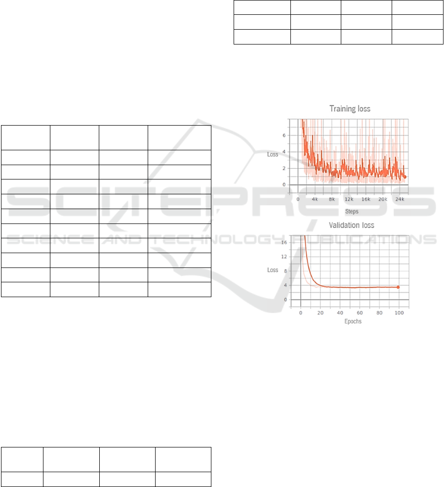
performance of the algorithm was registered. Table 2
reports the results obtained when optimizing the
dataset gradually with the goal of improving
performance.
Table 2: YOLOv3-tiny training results.
Training mAP FPS
Dataset
Images
1 88% 10 553
2 74% 29 1300
… … … …
9 93.1% 30 1090
10 93.0% 26.9 1090
11 93.7% 27.2 1110
12 91.5% 26.2 1110
… … … …
16 93.1% 26.5 1231
17
94.8%
26.4 1252
Analyzing the table, one can see the worse result
in the second train with mAP of 74%. This value was
caused by the shape inconsistency of the red and
white tape. Table 3 shows the details about the AP of
the red and white tape which proved to be the cause
of the mAP lowering. This tape proved to be
incredibly volatile regarding the deformation it
presents on every situation. Sometimes random and
similar objects mislead the algorithm and for that
reason it was replaced by the road separator.
Table 3: Red and White Tape training results.
Object Cone Sign
Red and
White Tape
AP 85.4% 100%
35.4%
For the next trainings the red and white tape was
disused due to low detection accuracy. Multiple
trainings were carried out to analyze the impact of
some changes and improvements in the algorithm
with proper testing between every training. Finally,
the best results were obtained in training number 17.
Table 4 shows the details.
Table 4: Best training YOLOv3-tiny results.
Training Cone AP Sign AP Divider AP
16 84.1% 99.3% 95.8%
17 86.7% 99.3% 98.5%
Figure 11 shows the loss obtained in the 17th training.
The training loss is calculated for every step whereas
the validation loss is calculated every epoch. The
results show that the model is not overfitting.
Figure 11: Results of YOLOv3-tiny training loss.
At this point, the dataset was already good and
then the hyperparameters were slightly changed in
order to obtain some minor improvements. Those
changes didn’t result in better performance so the
values remained the same. Figure 12 combines four
samples from real-world YOLOv3-tiny testing. The
real-time detection was performing at approximately
12 FPS so the testing video was stuttering. To avoid
that, the detection was made every other frame and
the capturing frame rate increased to approximately
25 FPS, as shown on the top left corner of the samples
of figure 12.
ICAART 2022 - 14th International Conference on Agents and Artificial Intelligence
798
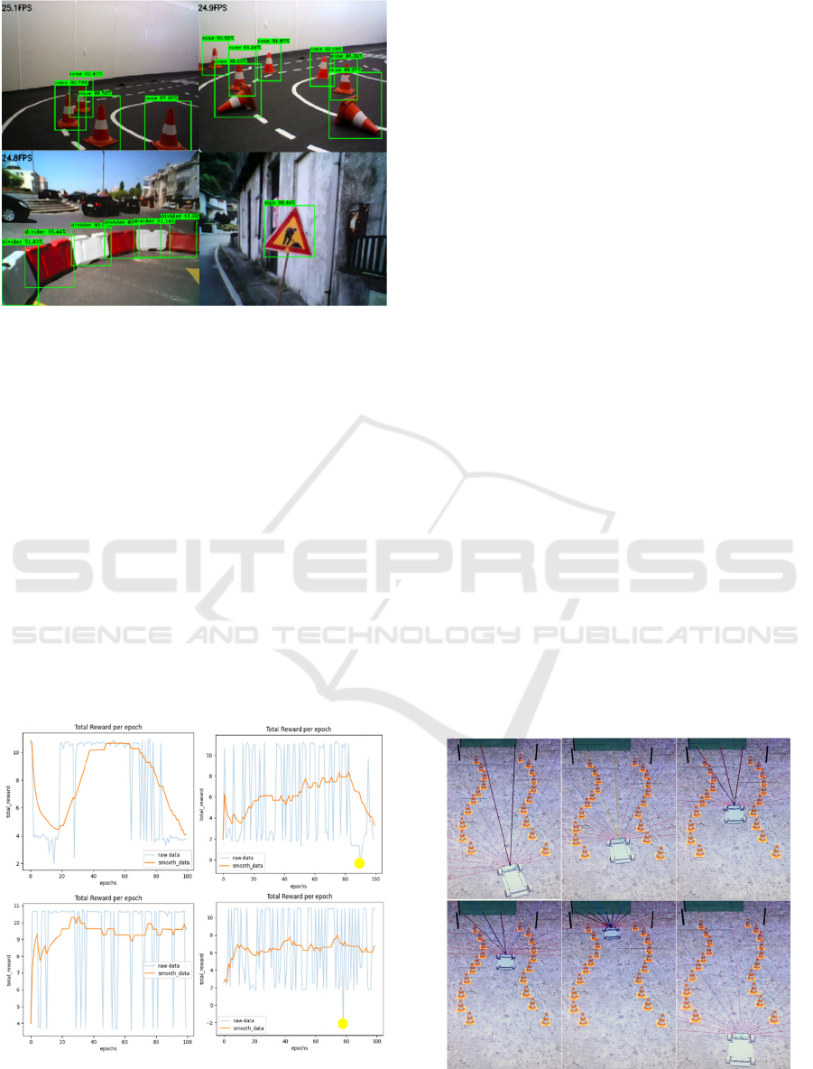
Figure 12: YOLOv3-tiny test with images captured from
real world.
In DDPG training, the exploration starts randomly
and so the algorithm results depend on the exploration
success. The list of hyperparameters along with its
chosen values is next described: Number of epochs =
100; Actor Learning Rate = 0.001; Critic Learning
Rate = 0.0001; OU theta = 0.15; OU sigma = 0.2;
Minibatch size = 64; Buffer size = 10000; Tau (used
to update target networks) = 0.001; Gamma= 0.99.
The neural networks of the DDPG approach consist
of two hidden layers with 400 and 300 neurons
respectively, with ReLU activation. follows the same
principle, using an output layer to compute the action
space for the actor network and the Q(s,a) pair for the
critic network. More than a hundred trainings were
performed and figure 13 shows the best results
achieved.
Figure 13: DDPG training and testing results obtained in
two different paths.
The top left graph represents the training for a
curved path and the bottom left graph represents the
correspondent test made. On the right side, the same
is true but for a double curved path. Both training and
testing graphs have a positive evolution along the
episodes. However, the training performance drops at
60 epochs on the curved path, and after the 80 epochs
for the double curved path. This phenomenon
occurred quite frequently and shows that DDPG can
unlearn the knowledge previously acquired.
To make sure the weights generated are not faulty
based on that phenomenon, checkpoints were
introduced to save them on the best learning point,
calculating the mean reward of the last 50 epochs. In
the case of the double curved path, once it reaches the
peak reward at 80 epochs, the mean value will be
higher and thus it will be the last checkpoint where
the weights are saved. Both testing graphs show an
average reward above 6. Therefore, most times it
performed the path with success, since approximately
every reward value of 10 represents the episode
completed with no faulty behaviors. Also, both
graphs show a negative peak almost at the end. The
negative peak, marked by a yellow dot, does not mean
that the vehicle did not go to the final line. Often
means that the vehicle decided to move very slowly
in the middle of the episode and the step variable on
the reward system ensures it gets penalized for it.
These peaks cannot be avoided since the algorithm
needs them to know that it is not a desirable behavior.
Figure 14 shows the vehicle completing the course
without any faulty behaviors, although as previous
graphs prove, this does not happen in 100% of the
cases and thus, it is still recommended for simulation
purposes only.
Figure 14: Demonstration of the vehicle using the
implemented system and completing the path.
Combining YOLO and Deep Reinforcement Learning for Autonomous Driving in Public Roadworks Scenarios
799

8 CONCLUSIONS
This project intended to show a proof of concept of
what can be achieved by integrating two different
types of neural networks learning methods regarding
autonomous driving. These cooperate and interact
with the environment where the system is trained and
tested. YOLOv3-tiny was used for detecting
roadworks signs and proved to have an mAP above
90%, so it is a good choice for real situations,
especially in autonomous driving where processing
speed is a major concern for maintaining safety.
DDPG was used for controlling the vehicle’s
behavior and showed to be well-qualified when
handling complex environments in simulation, since
it achieves the intended goal more than 50% of the
trials. At this point, it would not be recommended to
apply the system in real world yet, since it does not
perform as it should in 100% of the cases and that can
compromise the safety of the surrounding
environment or the passengers. The future work must
consist of continuously improving the two learning
methods to a point where both accuracy and safety are
reliable enough to transfer this autonomous driving
system to the real world.
ACKNOWLEDGMENTS
This work has been supported by FCT—Fundação
para a Ciência e Tecnologia within the R&D Units
Project Scope: UIDB/00319/2020. In addition,
this work has also been funded through a
doctoral scholarship from the Portuguese
Foundation for Science and Technology (Fundação
para a Ciência e a Tecnologia) [grant number
SFRH/BD/06944/2020], with funds from the
Portuguese Ministry of Science, Technology and
Higher Education and the European Social Fund
through the Programa Operacional do Capital
Humano (POCH).
REFERENCES
Adarsh, P., Rathi, P., & Kumar, M. (2020). YOLO v3-Tiny:
Object Detection and Recognition using one stage
improved model. 2020 6th IEEE (ICACCS).
https://doi.org/10.1109/icaccs48705.2020.9074315
Arcos-García, L., Álvarez-García, J. A., & Soria-Morillo,
L. M. (2018). Evaluation of deep neural networks for
traffic sign detection systems. Neurocomputing.
https://doi.org/10.1016/j.neucom.2018.08.0 09
Arcos-García, L., Álvarez-García, J. A., & Soria-Morillo,
L. M. (2018a). Deep neural network for traffic sign
recognition systems: An analysis of spatial
transformers and stochastic optimisation methods.
Neural Networks.https://doi.org/10.1016/j.neunet.2018
.01.005
Chun, D., Choi, J., Kim, H., & Lee, H. J. (2019). A Study
for Selecting the Best One-Stage Detector for
Autonomous Driving. 2019 34th ITC-CSCC.
https://doi.org/10.1109/itc-cscc.2019.8793291
Huang, Y., & Chen, Y. (2020). Autonomous Driving with
Deep Learning: A Survey of State-of-Art Technologies.
ArXiv. Published. http://arxiv.org/abs/2006.06091
Kaplan Berkaya, S., Gunduz, H., Ozsen, O., Akinlar, C., &
Gunal, S. (2016). On circular traffic sign detection and
recognition. Expert Systems with Applications, 48, 67–
75. https://doi.org/10.1016/j.eswa.2015.11.018
Kiran, B. R., Sobh, I., Talpaert, V., Mannion, P., Sallab, A.
A. A., Yogamani, S., & Perez, P. (2021). Deep
Reinforcement Learning for Autonomous Driving: A
Survey. IEEE ITS Transactions. https://doi.org/
10.1109/tits.2021.3054625
Lillicrap, T. P., Hunt, J. J., Pritzel, A., Heess, N., Erez, T.,
Tassa, Y., Silver, D. & Wierstra, D. (2016). Continuous
control with deep reinforcement learning.. In Y. Bengio
& Y. LeCun (eds.), ICLR.
Lim, K., Hong, Y., Choi, Y., & Byun, H. (2017). Real-time
traffic sign recognition based on a general purpose GPU
and deep-learning. PLOS ONE, 12(3), e0173317.
https://doi.org/10.1371/journal.pone.0173317
Liu, L., Lu, S., Zhong, R., Wu, B., Yao, Y., Zhang, Q., &
Shi, W. (2021). Computing Systems for Autonomous
Driving: State of the Art and Challenges. IEEE Internet
of Things Journal, 8(8), 6469–6486.
https://doi.org/10.1109/jiot.2020.3043716
Redmon, J., & Farhadi, A. (2018). YOLOv3: An
Incremental Improvement. ArXiv:1804.02767.
Ribeiro, T., Goncalves, F., Garcia, I., Lopes, G., & Ribeiro,
A. F. (2019). Q-Learning for Autonomous Mobile
Robot Obstacle Avoidance. 2019 IEEE (ICARSC).
https://doi.org/10.1109/icarsc.2019.8733621
Sallab, A., Abdou, M., Perot, E., & Yogamani, S. (2017).
Deep Reinforcement Learning framework for
Autonomous Driving. Electronic Imaging, 7076.
https://doi.org/10.2352/issn.24701173.2017.19.avm-
023
Svecovs, M., & Hörnschemeyer, F. (2020). Real time object
localization based on computer vision (thesis).
Gothenburg, Sweden.
Wang, S., Jia, D., & Weng, X. (2018). Deep Reinforcement
Learning for Autonomous Driving. ArXiv:1811.11329.
Yurtsever, E., Lambert, J., Carballo, A., & Takeda, K.
(2020). A Survey of Autonomous Driving: Common
Practices and Emerging Technologies. IEEE Access, 8,
58443–58469. https://doi.org/10.1109/access.2020.298
3149
ICAART 2022 - 14th International Conference on Agents and Artificial Intelligence
800
