Understanding the Scene: Identifying the Proper Sensor Mix in Different

Weather Conditions

Ziad Elmassik

, Mohamed Sabry

and Amr El Mougy

Computer Science Department, German University in Cairo, Cairo, Egypt

Keywords:

Object Classiﬁcation, Classiﬁcation Performance, Sensor Fusion, Autonomous Vehicles.

Abstract:

Autonomous vehicles rely on a variety of sensors for accurate perception and understanding of the scene.

Behind these sensors, complex networks and systems perform the driving tasks. Data from the sensors is

constantly perturbed by various noise elements, which compromises the reliability of the vehicle’s perception

systems. Sensor fusion may be applied to overcome these challenges, especially when the data from the

different sensors lead to contradicting results. Nevertheless, weather conditions such as rain, snow, fog, and

direct sunlight have an impact on the quality of sensor data, in different ways. This challenge has not been

studied in depth, according to the best knowledge of the authors. Accordingly, this paper presents an extensive

study of perception systems under different weather conditions, using real-life datasets (nuScenes and the

CADCD). We identify a set of evaluation metrics and study the quality of data from different sensors in

different scenarios and conditions. Our performance analysis produces insight as to the proper sensor mix that

should be used in different weather conditions.

1 INTRODUCTION

Automated Driving Systems (ADSs) promote the

highest safety standards on the roads. According to

the deﬁnition of levels of automation by the Society of

Automotive Engineers (SAE), the highest automation

level (level 5) requires full understanding of the en-

vironment through sensors. The camera (monocular

or stereo) is considered the main sensor in ADS and

is usually accompanied with other sensing modalities

such as lidars and radars, which are capable of depth

estimation and 3D mapping.

Data from these sensors is either processed inde-

pendently or through fusion by the vehicle’s percep-

tion systems. This data is constantly perturbed by

naturally occurring noise elements, which reduces the

quality of the data and often leads to unreliable results

from the perception systems. Harsh weather con-

ditions lead to compounded effects, leading even to

completely blind perception in some scenarios. How-

ever, sensors are not affected in the same way by dif-

ferent weather conditions. For example, direct sun-

light has a negative impact on cameras but radars are

unaffected. Rain and snow have a negative impact

https://orcid.org/0000-0001-9044-7460

https://orcid.org/0000-0002-9721-6291

https://orcid.org/0000-0003-0250-0984

on cameras and lidars, but radars are not affected as

much. Fog may reduce the visibility of cameras but

not lidars and radars.

Accordingly, it is important to have an accurate

evaluation of the quality of sensor data in different

conditions, in order to identify the proper sensor mix

that should be used in real-time. This is especially

important in sensor fusion, where compromised sen-

sor data may lead to contradicting results.

This paper presents an in-depth examination of

the performance of perception systems in different

weather conditions. We consider different sensors

such cameras, lidars, and radars, and we evaluate the

quality of the data from these sensors individually and

in fusion systems. We identify a comprehensive list of

metrics that evaluate the performance of the sensors

themselves as well as the perception systems. Our

evaluation produces signiﬁcant insight into how the

quality of sensor data degrades in different conditions.

We use the nuScenes dataset and the Canadian Ad-

verse Weather Conditions Dataset (CADCD) for our

performance analysis, as it includes a variety of sce-

narios and weather conditions that are of interest to

our study.

The remainder of this paper is structured follows:

In Section 2 some preliminary knowledge needed to

understand the work in this paper will be introduced.

Elmassik, Z., Sabry, M. and El Mougy, A.

Understanding the Scene: Identifying the Proper Sensor Mix in Different Weather Conditions.

DOI: 10.5220/0010911900003116

In Proceedings of the 14th International Conference on Agents and Artiﬁcial Intelligence (ICAART 2022) - Volume 3, pages 785-792

ISBN: 978-989-758-547-0; ISSN: 2184-433X

785

Section 3 presents the methodology of the work and

the details of our study. Following this, the results

of the work and discussed. Finally, the paper is con-

cluded in Section 5.

2 LITERATURE REVIEW

This section discusses multiple studies on the effects

of adverse weather conditions on sensor modalities.

Among them, (Heinzler et al., 2019) produced a thor-

ough analysis on the effects of harsh weather condi-

tions such as heavy rain and dense fog on lidar per-

formance. The authors also propose an approach to

detect and classify rain or fog only through the use

of lidar sensors. Results indicate mean union over in-

tersection of 97.14%. (Peynot et al., 2009), also pro-

vided insight on weather effects by recording a dataset

using camera, infrared camera, lidar, and radar sen-

sors in harsh environments. Results indicate that lidar

performs poorly in comparison to radar. Here, ob-

ject detection was used as a benchmark for evaluat-

ing sensor performance. (Hendrycks and Dietterich,

2019) perform bench-markings of object detectors

on images from a camera containing a multitude of

adverse weather conditions and found an approach

to improve robustness to such adversity. (Michaelis

et al., 2019) also, provided a benchmark of object de-

tectors on camera images containing adverse weather

conditions. Results indicated a decrease in model per-

formance from 60% to 30% of the original perfor-

mance. They also proposed a technique to pre-process

the images, thus increasing performance by a substan-

tial amount. (Lee et al., 2018) combined the data from

lidar, camera and GPS to create a real-time lane detec-

tion system, robust to adverse weather.

(Tang et al., 2019) proposed an autonomous sys-

tem capable of performing both localization and clas-

siﬁcation on a 5G network, with localization perform-

ing at 18 fps and classiﬁcation at 10. However, the

used modalities were not diverse enough.

In this work, multiple sensor modalities will be

tested on the multitude of weather conditions. Also,

all weather conditions in the previous works were em-

ulated in some form or another. For example, (Bijelic

et al., 2018) tested on fog, from a fog chamber, and

not on the actual road. In this work, testing is done on

weather conditions recorded on the open road, where

cars and pedestrians are present. Finally, this work

will investigate the best efﬁcient use of the sensor

conﬁguration based on the weather situation.

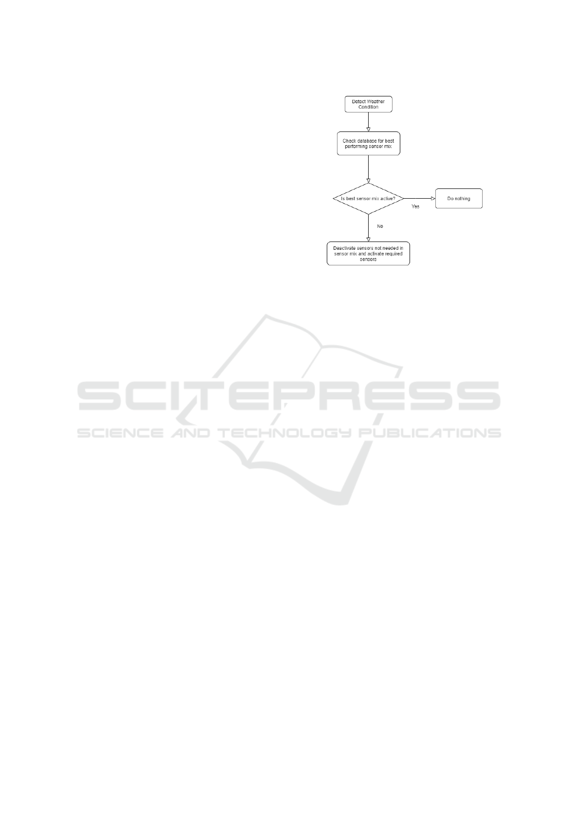
Figure 1: Flowchart for autonomous sensor activa-

tion/deactivation.

3 METHODOLOGY

The aim of this work is to assign the best perform-

ing sensor modality to a certain weather condition that

will perform with the best efﬁciency.

Therefore, given a certain weather condition,

computational requirements and power consumption

can be reduced by keeping the best performing mix of

sensors active, while deactivating the weaker ones. A

ﬂow of the system can be seen in 1. The weather con-

ditions upon which sensor conﬁgurations were tested

include cloudy , rain, and snow.

A virtual architecture in which a car is equipped

with 5 different sensors is introduced: 1. A single

monocular camera at the front, 2. A lidar on the roof

of the car, 3. A radar at the front located, 4. An IMU

and a GPS.

3.1 Identifying the Best Sensor

Conﬁguration per Weather

Condition

In order to produce quantiﬁable comparison results

for the sensors, different object classiﬁcation models

are used, in which each model would be assigned as a

representative for a sensor mix. Therefore, the accu-

racy shown by the model in a certain weather condi-

tion would be used to quantify the performance of the

sensor mix in that weather condition.

3.1.1 Choice of Sensor Mixes

In this section, the utilized sensor mixes will be dis-

cussed.

ICAART 2022 - 14th International Conference on Agents and Artiﬁcial Intelligence

786

The ﬁrst sensor mix involves the early fusion be-

tween the camera and the lidar sensors. The reason for

this is to compensate for the camera’s lack of depth

and difﬁculty in estimating 3D dimensions. The rea-

son why early fusion was chosen was because it re-

tains all data between the two sensors, unlike late fu-

sion which may lose features.

The second sensor setup is composed of a cam-

era and the third sensor setup is a single lidar. This

is to test their individual performance and compare

them to early fusion approaches. The objective here

is to evaluate whether noise on one sensor may signif-

icantly degrade early sensor fusion models, leading to

even worse performance than individual sensors.

The ﬁnal sensor mix is the middle fusion between

camera and radar. The radar is the only sensor unaf-

fected by weather conditions due to its use of radio

signals. However, its data is far too sparse to be used

on its own and must be fused with a different modal-

ity to add resolution. The camera was chosen as that

modality, as it has the highest resolution among all

sensors and can therefore compensate for the radar

pointcloud’s low resolution, while providing the cam-

era with depth perception.

The full camera-lidar-radar fusion was not pro-

posed, as it contradicts the purpose of the paper which

is to deactivate sensors for the goal of limiting com-

putation.

3.2 Datasets Used

Adverse weather conditions are rare to come across

in most datasets. This is especially prevalent

in the state-of-the-art datasets such as, PASCAL

VOC(Everingham et al., 2010) and KITTI(Geiger

et al., 2012) which are recorded in clear weather con-

ditions. Even nuScenes contains only one of the three

weather conditions desired for evaluation, which is

rain. In order to cover the three weather conditions

needed for generalization, a third dataset was used

known as the Canadian Adverse Driving Conditions

Dataset (CADCD). In this section, the datasets used

in this work along with their purpose are covered as

follows:

1. KITTI: Around 550 samples from the ofﬁcial

KITTI(Geiger et al., 2012) validation split were

chosen in an attempt to create a balance between

the occurrences of cars and pedestrians in clear

weather conditions.

2. NuScenes: Around 1100 samples combining

rainy and clear weather conditions from the of-

ﬁcial NuScenes (Caesar et al., 2020).

3. CADCD: Around 1650 samples combining

cloudy, rainy and snowy conditions in total from

CADCD(Pitropov et al., 2021).

3.3 Object Classiﬁcation Models Used

For evaluating the accuracy of the 4 sensor mixes in-

cluded in this paper, 4 different object classiﬁers uti-

lizing different modalities were chosen. All the mod-

els chosen are capable of achieving state-of-the-art

accuracy in comparison to others utilizing the same

sensor(s). The assignments are as follows:

• Lidar(Only)—SECOND(Yan et al., 2018): De-

fault settings set by mmdetection3D (Contribu-

tors, 2020).

• Camera(Only)—Faster R-CNN(Ren et al., 2015):

Default settings set by mmdetection (Chen et al.,

2019).

• Camera-Lidar—MVXNet(Sindagi et al., 2019):

Modiﬁed to read only 32 lidar channels/rings

(CADCD(Pitropov et al., 2021) utilizes a 32-ring

lidar). The same conﬁguration was used for evalu-

ating on KITTI(Geiger et al., 2012) for a fair com-

parison (MVXNet reads only 32 rings from the 64

emitted by the lidar used in KITTI).

• Camera-Radar—CenterFusion(Nabati and Qi,

2021): Modiﬁed the number of camera-radar

pairs to evaluate on to only 1 pair from the default

3.4 Dataset Preparation

To ensure a fair quantitative comparison, all the labels

of the datasets were converted to the KITTI dataset

label format. For the CADCD case, the 3D labels

are in the format: [label, position:{x,y,z}, dimen-

sions:{x,y,z}, yaw], where label is the class of the

object, the position represents the center of the object

within the lidar frame(x,y,z), the dimensions represent

the dimensions of the cube(x is width, y is length, z

is height), and yaw is the rotation around the vertical

axis.

In KITTI, the labels are represented as:

[type, truncated, occluded, alpha, bbox:{x

min

max

},dimensions:{y,z,x}, location:{x,y,z},

rotation

]. The type indicates the object category

namely cars and pedestrians. Truncation refers to

the object exiting the image boundaries. Occlusion

indicates how obstructed an object is. It is of no

relevance as the CADCD was recorded without

taking occlusion into account. Thus, it is set to

”fully visible” during conversion for all objects. The

alpha refers to the observation angle of the object

and it is between −π and π. Bbox represents the

Understanding the Scene: Identifying the Proper Sensor Mix in Different Weather Conditions

787

2D bounding box around an object using x

min

, y

min

max

, y

max

. Dimensions represent the 3D dimensions,

however the ordering of the dimensions is different,

whereas the order in the CADCD was width(x),

length(y), height(z), and the ordering used by KITTI

is height(y), width(z), and length(x) for representing

dimensions. Location is the same as the CADCD’s

position and rotation

is the same as the yaw.

Another difference between the two datasets is

the label computation. The CADCD(Pitropov et al.,

2021) computes its labels and calibration matrices

with respect to the lidar frame, whereas KITTI(Geiger

et al., 2012) computes theirs with respect to the cam-

era frame. This means that the axis conventions

on which annotations and extrinsic matrices are pro-

duced are different. The axis for the lidar frame used

by the CADCD are as follows: x pointing forward, y

pointing left and z pointing up. In the KITTI dataset’s

camera frame, these are: x pointing right, y pointing

down, and z pointing forward. For visualising the cur-

rent state of the conversion, a repository dedicated to

visualizing data in the KITTI dataset was used.

From these results, it was deduced that a series of

axes transformations on the CADCD 3D labels and

the CADCD camera-lidar extrinsic matrix, would be

necessary.

3.4.1 Axes Transformation

From what is understood about the two axes con-

ventions used by KITTI and the CADCD, a trans-

formation matrix is created to be multiplied with 3D

bounding box position coordinates and the Euler an-

gles from which the extrinsic matrix is derived. It was

found that, if the CADCD axes were to rotate once

around the x-axis by pi/2 radians, followed by a rota-

tion around the y-axis by −pi/2 radians, the x would

end up pointing right, y pointing down and z pointing

forward.

These transformation matrices are then multiplied

in the order opposite to that of their creation, giv-

ing us the transformation matrix for transforming the

CADCD axes to their counterparts in KITTI.

Trans f ormMat = Rotation

∗ Rotation

(1)

3.4.2 Extrinsic Matrix Conversion

An extrinsic matrix represents the transformation be-

tween any two sensors in the 3D world, in which one

of the two is set as the reference. In order to recon-

struct the extrinsic matrix for the KITTI axes, reverse-

engineering of the current one is necessary.

In order to reconstruct the extrinsic matrix, it must

be broken down into the 3x3 rotation matrix and 3x1

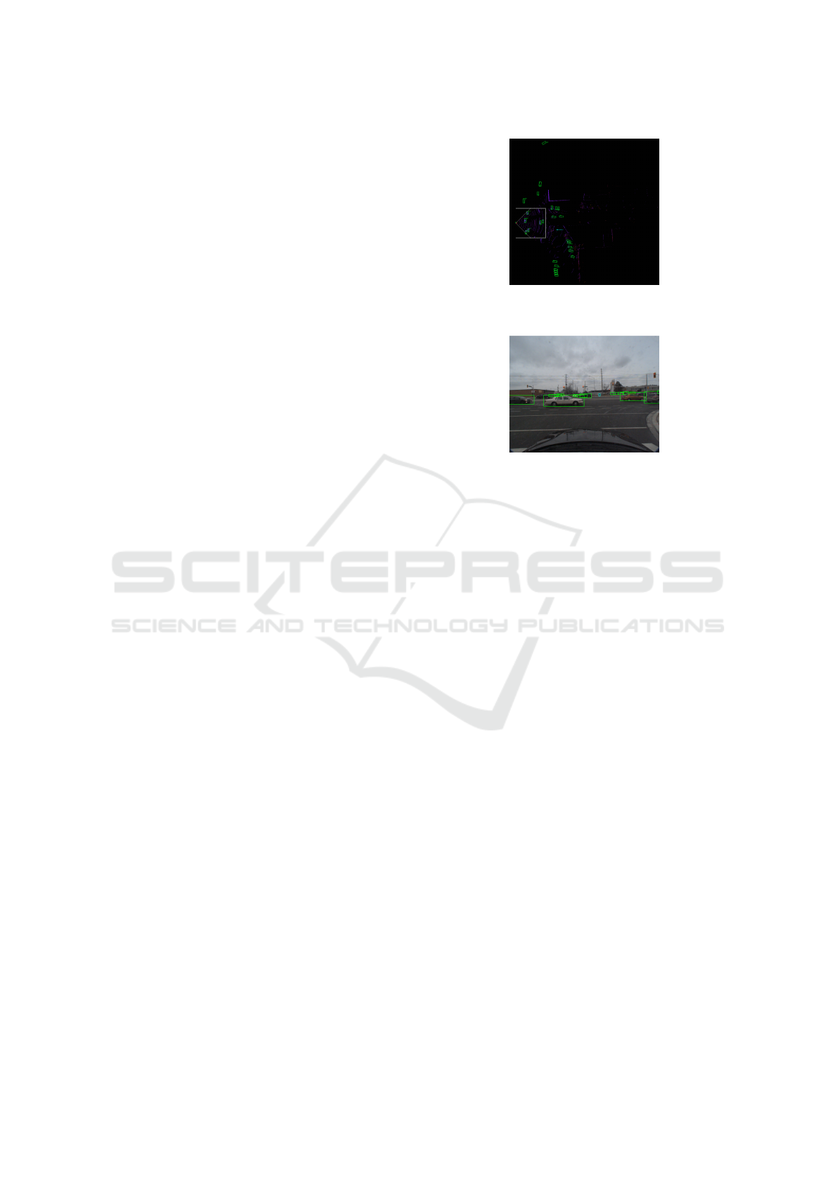
Figure 2: 3D Bounding Boxes existing outside of image

viewing frustum.

Figure 3: Generation of 2D ground truth.

vector as the translation matrix. Next, the three Euler

angles(roll, pitch, and yaw) are extracted from the ro-

tation matrix. After obtaining these Euler angles, they

are stored in a 3x1 vector and the 3x3 transformation

matrix, Trans f ormMat is multiplied by them provid-

ing the new angles. Delicate ﬁne-tuning of these two

parameters was applied to ensure a precise projection

of lidar to camera was attained on the new axes.

3.4.3 Location and Dimensions Conversion

The 3D labels must be properly aligned with the point

cloud to ensure the results are as accurate as possible.

For properly aligning the positions, the x,y, and z rep-

resenting the center of the object were stored into a

3x1 vector and once again, Trans f ormMat is multi-

plied by the vector creating new x, y, and z coordi-

nates for the new axes. Next, the dimensions needed

to be re-ordered from the CADCD’s width, length,

height to KITTI’s height, width, length.

3.4.4 BBox Calculation

2D bounding box data will be needed when eval-

uating Faster R-CNN. Unlike KITTI, the CADCD

labels do not contain 2D bounding box data, x

min

max

. This meant that these parameters had

to be reconstructed from the existing 3D bounding

box data. The center of the 3D bounding box out-

putted post-conversion along with the re-ordered di-

mensions, were used to output the bottom left and top

right vertices of the 2D bounding box. The generated

2D boxes can be seen in 3.

ICAART 2022 - 14th International Conference on Agents and Artiﬁcial Intelligence

788

3.4.5 Alpha and Yaw

Alpha is calculated using the standard mathematical

approach. First, the viewing frustum angle is calcu-

lated using arctan(x/z) where x is the x-component of

the center of the 3D box and z is the corresponding

z-component. Arctan(x/z) is then subtracted from the

yaw angle of the box. Rotation

from the CADCD

label is taken as is in the KITTI label. Now, the ”di-

mensions”, ”location”, ”alpha” and ”yaw” arguments

are ready. However, there was still an issue regarding

the 3D bounding boxes. The CADCD recorded their

labels via lidar so some 3D bounding boxes were lo-

cated outside the image ﬁeld-of-view as can be seen

in . This was remedied using a process mentioned

below.

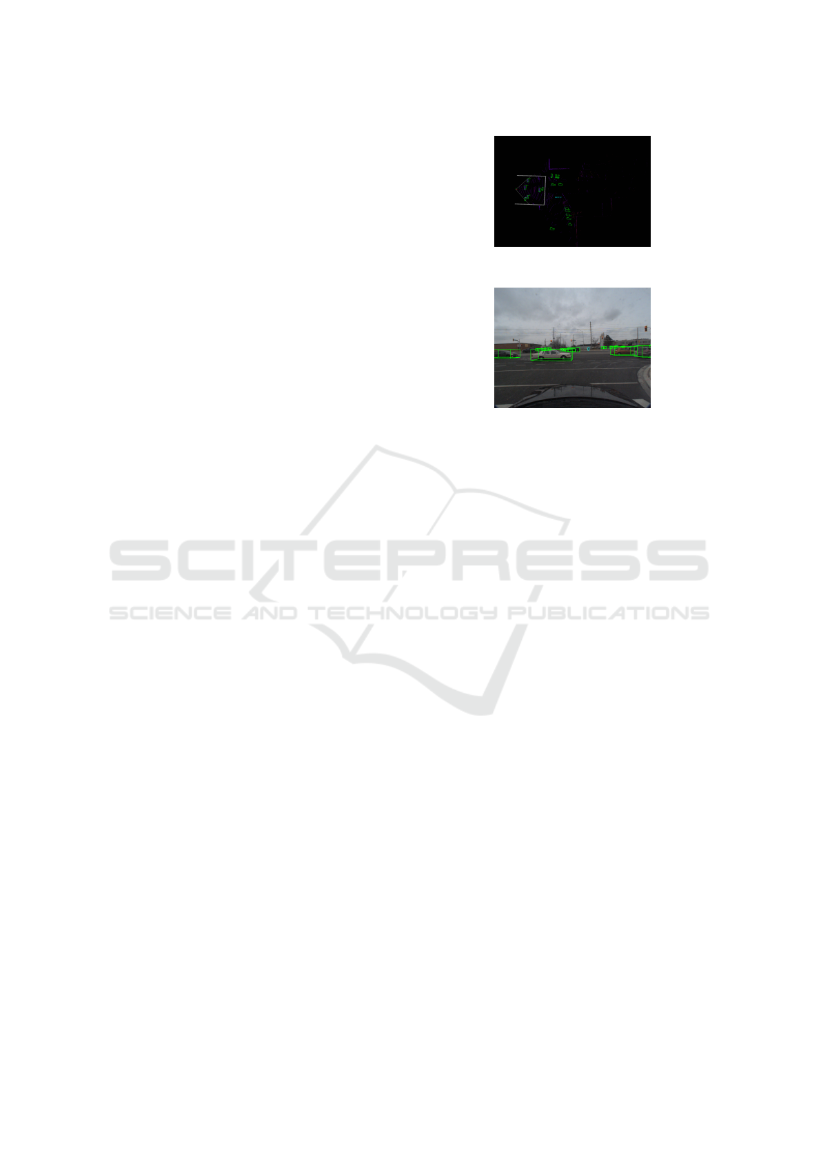
3.4.6 Truncation and Removing Out-of-View

Boxes

Truncation was calculated using a simple approach in-

volving the calculation of two different areas for the

bbox of an object, area-set and area-actual. For area-

set, four vertices are computed; x-min-set, y-min-set,

x-max-set, and y-max-set. X-min-set is computed, by

taking the maximum between 0 and the actual x

min

the bbox, then taking the minimum between this max-

imum and the image/frame width. The same is done

for x-max-set, except the maximum between 0 and

the actual x

max

is taken then the minimum is taken.

y-min-set and y-max-set follow the same approach in

which the maximum is taken between 0 and their ac-

tual counterparts and the minimum is taken between

the image height and the maximum. Finally, area-set

is computed by subtracting y-min-set from y-max-set

and the same is done for x then the two differences are

multiplied. What this approach does, is that in case of

truncation, it crops out the area of the bbox that is

outside the image, leaving only the area inside. The

corresponding set of areas(area-actual) is computed

for each bounding box by taking the area of the box

using the previously calculated, x

min

, y

min

max

Finally, the ratio area-set/area-actual is computed and

truncation is calculated by subtracting this ratio from

1, returning either a 0 or a 1.

For removing 3D boxes outside of the cameras’

FOV, a check is performed on area-set. If it is equal to

0, then this box is skipped. The result of this approach

is shown in 4 and 5.

3.4.7 Labels

Due to the conversion, only the 2 classes, car and

pedestrian were kept. The rest were lost, as KITTI

does not contain them in its labels.

Figure 4: Only 3D boxes inside viewing frustum are kept.

Figure 5: 3D boxes projected on the image within visu-

aliser, using new extrinsic matrix.

3.5 PASCAL VOC Conversion

For evaluating Faster R-CNN which loads data in

PASCAL VOC(Everingham et al., 2010) format. An

online repository known as vod-converter was used to

convert the new CADCD(Pitropov et al., 2021) labels,

in the form of KITTI(Geiger et al., 2012) to PASCAL

VOC(Everingham et al., 2010) labels.

4 RESULTS AND DISCUSSION

In this section, the results provided by the 4 differ-

ent sensor conﬁgurations(i.e. the object classiﬁca-

tion models representing them) are covered and com-

pared against those of their peers. The results are

categorized into 4 different weather conditions: clear,

cloudy, rain and snow.

A roughly equal number of samples containing

weather conditions were used during testing (approx.

550). Two classes were tested for classiﬁcation(car

and pedestrian). All samples were hand-picked for

balance between occurrences of cars and pedestrians.

All samples were taken from the validation splits of

their datasets. All weather conditions were used for

testing on all sensor conﬁgurations except CenterFu-

sion(Nabati and Qi, 2021) which was only tested on

clear and rainy samples. IoU threshold was ﬁxed at

50% for all tests except CenterFusion(mentioned in

chapter 3). Sensor conﬁgurations are ranked in terms

of accuracy, in each weather condition. Quantitative

results are in AP and qualitative results are also in-

cluded. Also please note: if a qualitative result ap-

Understanding the Scene: Identifying the Proper Sensor Mix in Different Weather Conditions

789

pears cropped, it is because no more predictions were

beyond the cropped region.

4.1 Metrics

4.1.1 Object Classes

For evaluating model accuracy, state-of-the-art met-

rics proposed by PASCAL VOC(Everingham et al.,

2010) and KITTI(Geiger et al., 2012) are used. From

the PASCAL VOC Dataset, the metric AP is used. It

is calculated for two different object classes, car and

pedestrian/person. Results of each model per class

are compared with other models for that same class.

The reason why only 2 classes were chosen will be

covered later.

4.1.2 Ensuring a Fair Comparison

For maintaining a fair comparison between the differ-

ent models, the following is done:

• All results are computed at an IoU threshold of

50% following the reasoning of the PASCAL

VOC dataset(Everingham et al., 2010). There

was however, the inconvenience of one of the

models being pre-trained on nuScenes and out-

putting results in the format of nuScenes which

use a different metric for setting overlap thresh-

olds(mentioned in Chapter 2). This could not be

avoided.

• For results outputted by models pre-trained on

KITTI, only the results for the ”moderate” dif-

ﬁculty were chosen as it is the average between

”easy” and ”hard” difﬁculties in terms of bound-

ing box height, occlusion, and truncation.

• A roughly equal number of samples was used

to represent different weather conditions with all

weather conditions being represented by approxi-

mately, 550 samples each. The reason behind this

value is discussed later.

4.2 Clear Weather

In this section, object classiﬁers in clear, optimal con-

ditions are evaluated and compared.

4.2.1 LiDAR-ONLY (SECOND)

SECOND was able to obtain mAP =74.2 on clear

weather conditions.

4.2.2 Camera-ONLY (Faster R-CNN)

The results of Faster R-CNN indicate mAP=56.15.

Qualitative results can be seen in 6.

Figure 6: Faster R-CNN accuracy on clear weather.

4.2.3 Camera-LiDAR (MVXNet)

MVXNet achieves mAP=66.97. Qualitative results

are shown in 7. There are many false positives.

Figure 7: MVXNet on clear weather conditions.

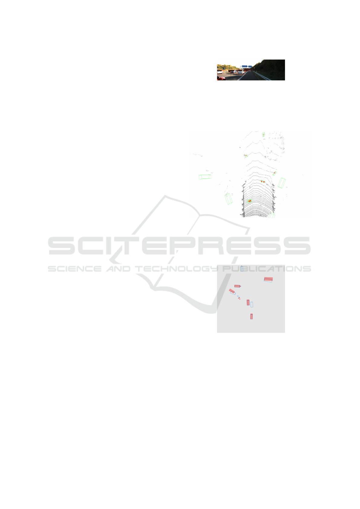
4.2.4 Camera-Radar (CenterFusion)

CenterFusion was able to achieve mAP = 47.1. Qual-

itative results can be seen in 8.

Figure 8: CenterFusion on clear weather conditions. Red

boxes indicate ground truth and cyan indicate predictions.

4.2.5 Rankings

From the results seen, it appears that the rankings are

as follows:

1. Lidar-only— mAP =74.2

2. Camera-lidar— mAP =66.97

3. Camera-only— mAP =56.15

4. Camera-Radar— mAP =47.1

ICAART 2022 - 14th International Conference on Agents and Artiﬁcial Intelligence

790

4.3 Cloudy Weather

In this section, the different sensor conﬁgurations are

tested on cloudy conditions.

4.3.1 Lidar-ONLY (SECOND)

The performance of SECOND was degraded resulting

in mAP=36.6. The results of the classiﬁcation were

acceptable when objects are within a close range from

the lidar.

4.3.2 Camera-ONLY (Faster R-CNN)

In the case of Faster R-CNN it got mAP=20.6. In this

case there was a large number of false negatives.

4.3.3 Camera-LiDAR (MVXNet)

MVXNet achieved mAP=20.5 in the cloudy weather.

In this case multiple false negatives were detected and

none of the pedestrians were detected. Orientation

estimation is also ﬂawed.

4.3.4 Rankings

Given the previous results, the rankings are as fol-

lows:

1. LiDAR-ONLY— mAP=36.6

2. Camera-ONLY— mAP=20.6

3. Camera-LiDAR— mAP=20.5

4.4 Rain

In this section, the different sensor conﬁgurations are

tested in rain.

4.4.1 Lidar-ONLY (SECOND)

SECOND yielded very low accuracy when detecting

pedestrians and mAP=10. There were numerous false

negatives with some false positives. There were ﬂaws

in orientation accuracy as well.

4.4.2 Camera-ONLY (Faster R-CNN)

A mAP=17.85 was achieved. There are balanced

detection rates between car and pedestrian classes.

Qualitative results were seen as poor with large

amounts of false negatives.

4.4.3 Camera-Lidar (MVXNet)

A mAP=10.6 was achieved. Results indicate multiple

false negatives, poor orientation prediction as well as

poor detection of pedestrians.

4.4.4 Camera-Radar (CenterFusion)

A robust detection was obtained in comparison to the

others with mAP=47.1 with very little offset between

the ground truth and the predictions.

4.4.5 Ranking

From the given results, the following rankings are

produced:

1. Camera-Radar mAP=47.1

2. Camera-ONLY mAP=17.85

3. Camera-Lidar mAP=10.6

4. Lidar-ONLY mAP=10

4.5 Snow

4.5.1 Lidar-ONLY (SECOND)

An accuracy of mAP = 32.99 with 0 accuracy for

pedestrians was obtained. Poor orientation estimation

was visible as well as multiple pedestrians being de-

tected as cars.

4.5.2 Camera-ONLY (Faster R-CNN)

A mAP of 21 was indicated. Qualitative results indi-

cate adequate pedestrian detection.

4.5.3 Camera-Lidar (MVXNet)

A mAP=23.93 was obtained with 0% accuracy in de-

tecting pedestrians. Qualitative results indicated poor

orientation estimation, as well as many missing detec-

tions.

4.5.4 Ranking

Even though lidar and camera-lidar indicate better

higher mAP than camera-only, camera-only will be

ranked ﬁrst as it is the only conﬁguration that has

pedestrian detection accuracy exceeding 0%.

1. Camera-ONLY mAP=21

2. Lidar-ONLY mAP=32.99

3. Camera-Lidar mAP=23.93

4.6 Final Rankings

Now that all sensor conﬁgurations have been ranked

on all weather conditions, it is time to display the best

sensor conﬁguration for each weather condition.

Understanding the Scene: Identifying the Proper Sensor Mix in Different Weather Conditions

791

1. For Clear Weather: Lidar-ONLY

2. For Cloudy Weather: Lidar-ONLY

3. For Rainy Weather: Camera-Radar

4. For Snowy Weather: Camera-ONLY

However, given the fact that rain and snow pro-

duce similar types of noise, an assumption can be

made that camera-radar may be the best for snowy

conditions, as well as rain.

5 CONCLUSION

In this paper, various datasets containing various

weather conditions were used and tested on different

modalities for the goal of ﬁnding the best sensor con-

ﬁguration for each weather condition. From the eval-

uations of the different sensor modalities, insight as

to which sensors should be used for which weather

conditions has been gained. Now, preparations can be

made for the next step which is to develop a frame-

work based on this knowledge, then an efﬁcient and

safe system for computation on edge devices may be

developed.

Future work opportunities may include the addi-

tion of a model for classifying weather conditions, so

that the decisions can be made based on the model’s

output. A variety of conﬁgurations utilizing different

modalities was tested in this paper. However, there

may still be some novel sensors that can be tested

such as, thermal cameras and night-vision cameras.

Also, camera-radar fusion was only tested on clear

and rainy conditions. An opportunity would be to

test this fusion on other conditions. Moreover, this

work resorted to the evaluation of earlier fusion ap-

proaches between sensors(early and middle). Testing

of late-fusion architectures may add more insight as

to which sensor conﬁguration is best-suited to each

weather condition. Finally, it may be beneﬁcial to test

on a large amount of samples.

REFERENCES

Bijelic, M., Gruber, T., and Ritter, W. (2018). Benchmark-

ing image sensors under adverse weather conditions

for autonomous driving. 2018 IEEE Intelligent Vehi-

cles Symposium (IV), pages 1773–1779.

Caesar, H., Bankiti, V., Lang, A. H., Vora, S., Liong, V. E.,

Xu, Q., Krishnan, A., Pan, Y., Baldan, G., and Bei-

jbom, O. (2020). nuscenes: A multimodal dataset

for autonomous driving. 2020 IEEE/CVF Conference

on Computer Vision and Pattern Recognition (CVPR),

pages 11618–11628.

Chen, K., Wang, J., Pang, J., Cao, Y., Xiong, Y., Li, X.,

Sun, S., Feng, W., Liu, Z., Xu, J., Zhang, Z., Cheng,

D., Zhu, C., Cheng, T., Zhao, Q., Li, B., Lu, X., Zhu,

R., Wu, Y., Dai, J., Wang, J., Shi, J., Ouyang, W., Loy,

C. C., and Lin, D. (2019). MMDetection: Open mm-

lab detection toolbox and benchmark. arXiv preprint

arXiv:1906.07155.

Contributors, M. (2020). MMDetection3D: OpenMMLab

next-generation platform for general 3D object detec-

tion. https://github.com/open-mmlab/mmdetection3d.

Everingham, M., Gool, L., Williams, C. K., Winn, J.,

and Zisserman, A. (2010). The pascal visual ob-

ject classes (voc) challenge. Int. J. Comput. Vision,

88(2):303–338.

Geiger, A., Lenz, P., and Urtasun, R. (2012). Are we ready

for autonomous driving? the kitti vision benchmark

suite. In 2012 IEEE Conference on Computer Vision

and Pattern Recognition, pages 3354–3361.

Heinzler, R., Schindler, P., Seekircher, J., Ritter, W., and

Stork, W. (2019). Weather inﬂuence and classiﬁcation

with automotive lidar sensors. In 2019 IEEE Intelli-

gent Vehicles Symposium (IV), pages 1527–1534.

Hendrycks, D. and Dietterich, T. G. (2019). Benchmarking

neural network robustness to common corruptions and

perturbations. ArXiv, abs/1903.12261.

Lee, U., Jung, J., Jung, S., and Shim, D. (2018). Develop-

ment of a self-driving car that can handle the adverse

weather. International Journal of Automotive Tech-

nology, 19:191–197.

Michaelis, C., Mitzkus, B., Geirhos, R., Rusak, E., Bring-

mann, O., Ecker, A. S., Bethge, M., and Brendel, W.

(2019). Benchmarking robustness in object detection:

Autonomous driving when winter is coming. ArXiv,

abs/1907.07484.

Nabati, R. and Qi, H. (2021). Centerfusion: Center-based

radar and camera fusion for 3d object detection. 2021

IEEE Winter Conference on Applications of Computer

Vision (WACV), pages 1526–1535.

Peynot, T., Underwood, J., and Scheding, S. (2009). To-

wards reliable perception for unmanned ground vehi-

cles in challenging conditions. In 2009 IEEE/RSJ In-

ternational Conference on Intelligent Robots and Sys-

tems, pages 1170–1176.

Pitropov, M., Garcia, D., Rebello, J., Smart, M., Wang, C.,

Czarnecki, K., and Waslander, S. L. (2021). Canadian

adverse driving conditions dataset. The International

Journal of Robotics Research, 40:681 – 690.

Ren, S., He, K., Girshick, R. B., and Sun, J. (2015). Faster

r-cnn: Towards real-time object detection with region

proposal networks. IEEE Transactions on Pattern

Analysis and Machine Intelligence, 39:1137–1149.

Sindagi, V. A., Zhou, Y., and Tuzel, O. (2019). Mvx-net:

Multimodal voxelnet for 3d object detection. 2019

International Conference on Robotics and Automation

(ICRA), pages 7276–7282.

Tang, J., Liu, S., Yu, B., and Shi, W. (2019). Pi-edge: A

low-power edge computing system for real-time au-

tonomous driving services. ArXiv, abs/1901.04978.

Yan, Y., Mao, Y., and Li, B. (2018). Second: Sparsely

embedded convolutional detection. Sensors (Basel,

Switzerland), 18.

ICAART 2022 - 14th International Conference on Agents and Artiﬁcial Intelligence

792