Parameter Setting in SAT Solver using Machine Learning Techniques

Filip Beskyd and Pavel Surynek

Faculty of Information Technology, Czech Technical University, Th

akurova 9, 160 00 Praha 6, Czech Republic

Keywords:

SAT Problem, Boolean Satisﬁability, Solver, Graph Structure, Machine Learning, Heuristic Parameter Tuning.

Abstract:

Boolean satisﬁability (SAT) solvers are essential tools for many domains in computer science and engineering.

Modern complete search-based SAT solvers represent a universal problem solving tool which often provide

higher efﬁciency than ad-hoc direct solving approaches. Over the course of at least two decades of SAT related

research, many variable and value selection heuristics were devised. Heuristics can usually be tuned by single

or multiple numerical parameters prior to executing the search process over the concrete SAT instance. In this

paper we present a machine learning approach that predicts the parameters of heuristic from the underlying

structure of the input SAT instance.

1 INTRODUCTION

The Boolean satisﬁability (SAT) problem, the task of

ﬁnding a truth-value assignment of a given Boolean

formula, is one of the fundamental computer science

problems (Biere et al., 2009). Concretely; the SAT

problem was the ﬁrst one to be proven to belong to the

NP-Complete class of problems (Cook, 1971). Major

direct use-cases of SAT come from industries such

as software testing (Dennis et al., 2006), automated

planning (Kautz and Selman, 1992), hardware ver-

iﬁcation (Gupta et al., 2006) or cryptography (Soos

et al., 2009), as well as many other. Moreover, many

other problems of computer science are often reduced

to SAT.

Standard and in practice often used way of solv-

ing a given problem is to compile it, in some way, to a

concrete SAT instance which is then given to another

program as an input, so called a SAT Solver. The

SAT solver solves the instance and answers whether

there exists a truth-value assignment by which it can

be satisﬁed or not, with the concrete proof, that is ei-

ther variables assignment which satisfy the formula or

conﬂict.

There exist many solvers to the SAT problem.

Solvers are divided into two major groups, local

search and systematic search solvers. This work

is focused on systematic search solvers based on

the Conﬂict-driven clause-learning (CDCL) algo-

rithm (Marques Silva and Sakallah, 1996) whose

https://orcid.org/0000-0001-7200-0542

implementations come as variants of the Minisat

(Niklas E

en, 2004) solver.

CDCL SAT solvers have witnessed dramatic im-

provements in their efﬁciency over the last 20 years,

and consequently have become drivers of progress in

many areas of computer science such as formal ver-

iﬁcation (Newsham et al., 2015). There is a general

agreement that these solvers somehow exploit struc-

ture inherent in industrial instances due to the clause

learning mechanism and its cooperation with variable

and value selection heuristics.

Typically, implementations of CDCL SAT solvers

have many parameters, such as variable decay, clause

decay and frequency of restarts, which need to be set

prior to the solver being executed. Depending on how

various parameters are set for an input instance of-

ten has signiﬁcant impact on the running time of the

solver. Hence it naturally makes sense to try to set

these parameters automatically.

The paper is organized as follows: in Section 3

we introduce related works, Section 4 states which

parameters will be tuned and brieﬂy explains their

meaning, Section 5 measures the impact of each pa-

rameter on solving time, Section 6 presents how we

applied machine learning to our problem and ﬁnally

in Section 7 we evaluate our machine learning param-

eter setting in various benchmarks.

586

Beskyd, F. and Surynek, P.

Parameter Setting in SAT Solver using Machine Learning Techniques.

DOI: 10.5220/0010910200003116

In Proceedings of the 14th International Conference on Agents and Artiﬁcial Intelligence (ICAART 2022) - Volume 2, pages 586-597

ISBN: 978-989-758-547-0; ISSN: 2184-433X

2 CONTRIBUTION

In this work we apply machine learning techniques

(Mitchell, 1997) to predict the values for the parame-

ters of SAT solver which reduce solving time, based

on the type of an input instance. This step is moti-

vated among else by notion that many instances for a

ﬁxed domain are in some way similar thus formula’s

hidden structure will be similar as well.

For example the structure of most industrial SAT

instances are vastly different from the structure of the

random SAT instances (Ans

otegui et al., 2012) or in-

stances constructed for planning problems, and these

are different from instances encoding puzzles like the

pigeon-hole problem. Problems that belong to the

same class tend to have similar structure within the

class and speciﬁc values of the parameters work bet-

ter for them, than having the default parameter setting

globally for every instance.

Our contribution presented in this paper consists

in:

1. Visual summary of dependencies of solving time

on setting of various parameters of the SAT solver.

2. Extending the set of usual features extracted

by SAT solvers from instances, by computing

graph related features on clause graph (CG), and

variable–clause graph (VCG), which ought to bet-

ter capture the underlying structure of the in-

stance.

3. Building a machine learning mechanism based

on the extended set of features that sets the SAT

solver’s parameters according to the input in-

stance.

3 RELATED WORK

3.1 Portfolio Solver: SatZilla

SatZilla (Xu et al., 2008) is a portfolio solver, which

won many awards in SAT Competition (SAT, ). It in-

troduced new approach of using many other solvers

(portfolio) in the background. The solvers are used

as-is, and SatZilla does not have any control over their

execution.

Machine learning was previously shown to be an

effective way to predict the runtime of SAT solvers,

and SatZilla exploits this. It uses machine learning to

predict hardness of the input instance, and then based

on this prediction select a solver from its portfolio

which will be assigned to solve the problem. This

works because different solvers are better for different

types of instances. Predicting hardness of an instance

is done by ﬁrst extracting various features from the

input.

To train the model, SatZilla will ﬁrst compute

some features on training set of problem instances and

run each algorithm in the portfolio to determine its

running times. When the new input instance comes,

it computes its features. These are then used as input

for predictive model which predicts the best solver to

be used. That particular solver is then used to solve

instance.

3.2 Parameter Tuning: AvatarSat

AvatarSat (Ganesh et al., 2009) is a modiﬁed version

of Minisat 2.0 which introduced two key novelties.

First one is that it used machine learning to de-

termine the best parameter settings for each SAT for-

mula.

Second novelty in AvatarSat is the ”course cor-

rection” as it dynamically ”corrects” the direction in

which solver is searching. Modern SAT solvers store

new learnt clauses and drop input clauses during the

search, which can change the structure of the problem

considerably. AvatarSat’s argument is that the opti-

mal parameter settings for this modiﬁed problem may

be signiﬁcantly different from the original input prob-

lem.

Input SAT instances are classiﬁed using 58 differ-

ent features of SAT formulas such as ratio between

variables and clauses, number of variables, number of

clauses, positive and negative literal occurrences etc.

AvatarSat is tuning only two parameters,

-var-decay and -rinc, nine values for the ﬁrst

one and three for the second one, so the number of

examined conﬁgurations is 27.

3.3 Iterated Local Search

The key idea underlying iterated local search is to fo-

cus the search not on the full space of all candidate so-

lutions but on the solutions that are returned by some

underlying algorithm, typically a local search heuris-

tic. (Lourenc¸o et al., 2010)

Iterated local search is a local search algorithm

that optimizes parameters but only one dimension at a

time, it is a one-dimensional variant of hill climbing.

In (Pintjuk, 2015) author has used this algorithm

for MiniSat’s parameter tuning. There was not feature

extraction approach as in AvatarSat, SatZilla and this

paper, but it was an attempt to tune SAT solvers pa-

rameters and therefore we mention his solution in this

chapter. Results were measured only on factorization

problem instances.

Parameter Setting in SAT Solver using Machine Learning Techniques

587

4 TUNED PARAMETERS

We will tune the following heuristics settings of Min-

iSat solver as these have the most signiﬁcant impact

on the solver’s running time.

• -var-decay the VSIDS’s decay factor

• -cla-decay the clause decay factor

• -rfirst base restart interval

• -rinc restart interval increase factor

4.1 VSIDS

VSIDS is an abbreviation of variable state indepen-

dent decaying sum. VSIDS has become a standard

choice for many popular SAT solvers, such as Min-

iSat (Niklas E

en, 2004) which we employed as default

solver for this paper.

The main idea of VSIDS heuristic is to associate

each variable with an activity, which signiﬁes a vari-

able’s frequency of appearing in recent conﬂicts via

the mechanism of bump and decay.

Bump is a number which is incremented by 1 ev-

ery time this variable appears in conﬂict.

Decay factor 0 < α < 1 is a number by which each

of the variable’s activity is multiplied after each con-

ﬂict and thus decreased.

4.2 Clause Decay

In MiniSat, similar principle as in VSIDS is applied

to clauses. When a learnt clause is used in the

conﬂict analysis, its activity is incremented. Inac-

tive clauses are periodically removed from the learnt

clauses database (Niklas E

en, 2004). Since a set

of unsatisﬁable clauses generates many conﬂicts, and

therefore many conﬂict clauses, the high activity of a

clause can be seen as a potential sign of unsatisﬁabil-

ity. (D’Ippolito et al., 2010)

4.3 Restart Frequency

Frequency of restarts in MiniSat is determined by two

parameters, the base restart interval and restart inter-

val increase factor. One round of search will take as

long until the search encounters given number of con-

ﬂicts L. For example, minisat(120) will be search-

ing space of assignments as long as it reaches count of

conﬂicts equal to 120. After that, the algorithm will

pause, determine new number of needed conﬂicts to

force next restart, and continue searching.

Number of needed conﬂicts to restart L is deter-

mined as follows:

L = restart base · restart inc factor

#restarts

5 IMPACT OF PARAMETERS

The term “structure”, due to its vagueness, leaves

much room for interpretation, though, and it remains

unclear how this structure manifests itself and how

exactly it should be exploited. (Sinz and Dieringer,

2005)

However, research has advanced since then, and

nowdays the structure of some instances can be ex-

ploited.

Base idea of this paper comes from (Ans

otegui

et al., 2012), where it was shown that industrial in-

stances exhibit ”hidden structures” based on which

solver is learning clauses during search. In (Pipatsri-

sawat and Darwiche, 2007) researchers have shown

that formulas with good community structure tend to

be easier to solve.

Variables form logical relationships and we hy-

pothesize that VSIDS exploit these relationships to

ﬁnd the variables that are most ”constrained” in the

formula. The logical relationship between variables

are concretized as some variation of the variable inci-

dence graph (VIG). (Liang, 2018)

Our idea is to exploit this fact, so we will construct

three types of graphs which are representing each

instance, compute various properties of this graph

which will be used as features for machine learning,

in addition to standard features of the instance like

number of variables, clauses, their ratios etc.

This section is dedicated to present results of our

initial data exploration. We performed several ob-

servations on four different classes of problems, on

which we observe how the solver’s parameters affect

then number of conﬂicts, and thus solving time.

5.1 Classes of Selected SAT Instances

In this paper we limited ourselves to the follow-

ing SAT problem’s structurally diverse classes, for

which we expected different demands on parameters.

• Random SAT/UNSAT

• Pigeonhole problem

• Planning

– n

− 1 problem

– Hanoi towers

• Factorization

Random SAT/UNSAT are instances of 3-SAT

problem, generated randomly. This class of problems

if used as benchmark in SAT competition, this the cat-

egory’s name is RANDOM.

Pigeonhole problem involves showing that it is

impossible to put n + 1 pigeons into n holes if

ICAART 2022 - 14th International Conference on Agents and Artiﬁcial Intelligence

588

each pigeon must go into a distinct hole. It is

well known that for this combinatorial problem there

is no polynomial-sized proof of the unsatisﬁabil-

ity. (Haken, 1984) Combinatorial problems are part

of SAT competition benchmarks as well, known as

CRAFTED. We chose pigeonhole problem as one rep-

resentative, because it can be generated easily with

random starting positions with ﬁxed size.

As Planning problems representatives we chose

problem known as n

− 1 problem, or in its ﬁxed size

(n = 4) form Lloyd’s ﬁfteen. We generated numbered

tiles order randomly, and aggregated these instances

always within ﬁxed size, E.g., we never combined

problem of size 4x4 with 5x5. Another representative

of planning is Hanoi towers problem, this problem is

not possible to ”randomize” because initial state is

always given, we included this problem to observe

whether it will exhibit similarities to our other plan-

ning problem.

Factorization problem is problem of determining

whether a big number is a prime. It is an example of

INDUSTRIAL instance from SAT competitions.

5.2 Correlation of Number of Conﬂicts

and Solving Time

For the initial dataset building process, it is necessary

to ﬁnd close to optimal solver parameters for which

the solving time is lowest possible.

Because some harder instances take several tens

of seconds to solve, it would be unfeasible to generate

dataset from solving each of these instances by brute

force search on grid of parameter values, thus we de-

cided to build this dataset from small instances from

SATLIB. These instances are usually solved within

fraction of second by Minisat solver, but this approach

comes with a trade-off, it is hard to capture real solv-

ing time, because for these small instances overhead

can outweigh useful computation time.

Solving time varies a bit with every run and

solving time captured by MiniSat also includes sev-

eral system-originated factors which are not desired.

However, computation is deterministic with ﬁxed ini-

tial random seed, so it is natural to use number of con-

ﬂicts as other metric instead of actual solving time.

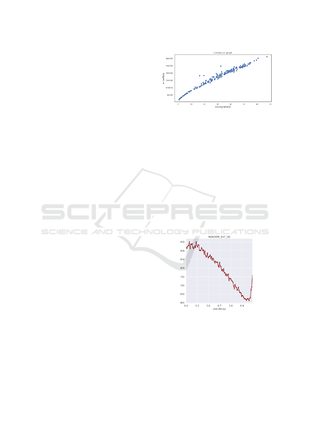
Scatter plot in Figure 1 shows strong correlation

between the number of conﬂicts and solving time on

randomly selected instances from SATLIB. As an im-

plication of this observation it is correct to use conﬂict

count as measurement of performance of the parame-

ters instead of time.

Figure 1: Correlation between number of conﬂicts and solv-

ing time.

5.3 Observed Parameters

Following subsections illustrate how number of con-

ﬂicts depends on selected parameters for each of

aforementioned problem classes. Note that axes do

not have same values in each of the examples. Before

we made these plots we ﬁrst analyzed which inter-

vals should we chose to discretize. E.g. we observed

that variable decay parameter for values in (0, 0.4)

always yielded bad results so we excluded those and

only examined [0.4,1). We have omitted label of ver-

tical axis, and it will always be number of conﬂicts.

Following plots in this section were ﬁrst aggre-

gated by different random seeds, and then aggregated

per many instances of the same size.

5.3.1 Variable Decay

Figure 2: Variable decay on random SAT instances.

For random satisﬁable instances shown in Figure 2

it seems that variable decay at around 0.95 gives best

results. For unsatisﬁable instances the plot is slightly

”smoother”, this is likely because the solver has to

search entire space so there are not many backjumps

which would cut ”heavy” branches.

From Figure 3 it seems that factorization instances

require -var-decay close to 1. Unsatisﬁable variant

(prime numbers) is smoother with the same result.

Parameter Setting in SAT Solver using Machine Learning Techniques

589

Figure 3: Variable decay on factorization instances.

(a) n

− 1 problem instances.

(b) Hanoi tower planning.

Figure 4: Variable decay on planning instances.

Figure 4 shows that planning instances are very

different from previous instances. As -var-decay

increases from 0.9 higher number of conﬂicts rises

rapidly, this may be signaling that planning instances

have variables which are more-less independent, be-

cause setting variable decay factor close to value of

1, effectively means algorithm will decay activity of

variables very slowly.

Behavior of pigeonhole problem instances was

identical to factorization.

5.3.2 Clause Decay

Figure 5: Clause decay on random SAT instances.

Figure 5 shows that it is best to set -cla-decay to

value very close to 1 for random instances.

(a) Satisﬁable.

(b) Unsatisﬁable.

Figure 6: Clause decay on factorization instances.

ICAART 2022 - 14th International Conference on Agents and Artiﬁcial Intelligence

590

Same conclusion can be seen in Figure 6 for fac-

torization instances, but the trend starts to decrease

signiﬁcantly at the value of 0.93.

For planning instances, we did not observe any de-

pendency, leading us to conclusion that -cla-decay

parameter does not have signiﬁcant impact.

Figure 7: Clause decay on pigeonhole instances.

For pigeonhole problem, Figure 7 shows similar

course as for random and factorization instances.

5.3.3 Restart Interval Increase Factor

In Figure 8, higher value seems to be better for ran-

dom instance, but important note is that the instances

on which we performed these aggregations are of

smaller size than in SAT competitions (SAT, ). For

those, these plots could look very different. We hy-

pothesize that for big instances smaller value of this

parameter would be better, because if the value is too

high, it might mean that longer the solver is running,

the interval until next restart will be too high, so the

much needed restart would not happen in very long

time.

In Figure 9, for not prime instances it was unclear

what value could be suitable, prime instances show

that values above 10 seems to be fastest.

For planning instances, it is clear from Figure 10

that lower values yield faster solving. There is raising

trend, but we think this is dependent on instance size.

Lower value means more frequent restarts, that is sug-

gesting that solver is often in local optima, which

eventually will not lead to solution and the restart

is needed. Hanoi tower problem also required very

small value, dependency on this parameter was almost

linear.

Plot in Figure 11 shows that for value 5 and higher

impact of this parameter does not yield any signiﬁcant

improvement. Higher values are preferred for pigeon-

hole problem, this means that the problem demands

less restarts because it is likely doing useful work, in

(a) Satisﬁable.

(b) Unsatisﬁable.

Figure 8: Restart interval increase factor on random SAT

instances.

Figure 9: Restart interval increase factor on factorization

instances.

other words, the path to solution is narrow so there are

not many branches which lead to local optima.

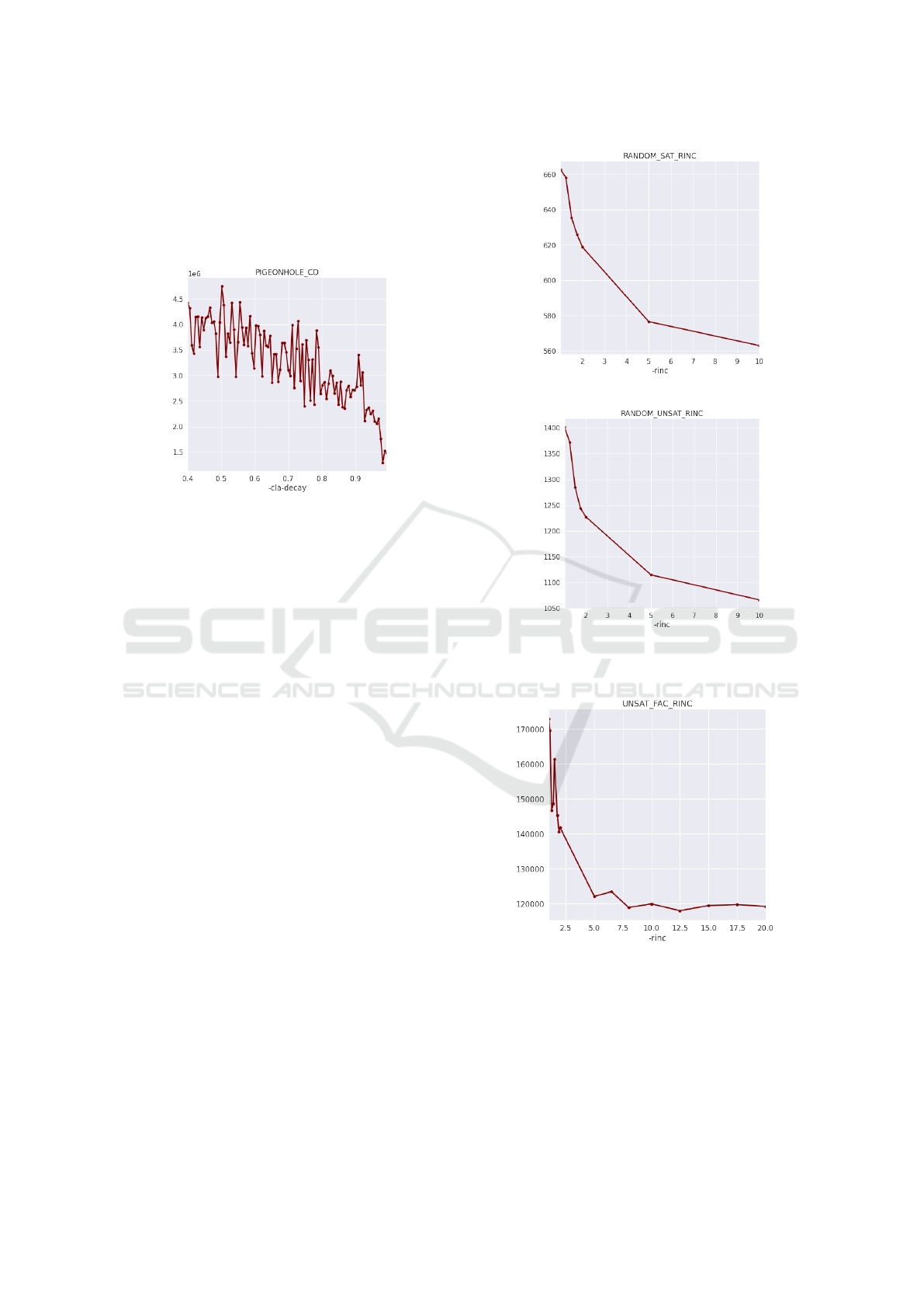
5.3.4 Restart Interval Base

Figure 12 shows that initial restart interval around 200

conﬂicts seems best for both satisﬁable and unsatisﬁ-

Parameter Setting in SAT Solver using Machine Learning Techniques

591

Figure 10: Restart interval increase factor on planning in-

stances.

Figure 11: Restart interval increase factor on pigeonhole

instances.

Figure 12: Restart interval base on random SAT instances.

able random instances, this is dependent on the size

of the problem.

We did not observe any dependency of -rfirst

factorization instances.

Figure 13: Restart interval base on planning instances.

Both plots in Figure 13 contain increasing trend

despite plot lines are quite different, so for planning

instances smaller initial interval is to be preferred, and

thus more frequent restarts.

Figure 14: Restart interval base on pigeonhole instances.

Decreasing trend in Figure 14 suggests that less

frequent intervals perform better for pigeonhole in-

stances, this further conﬁrms the hypothesis made

ICAART 2022 - 14th International Conference on Agents and Artiﬁcial Intelligence

592

with restart increase factor in previous section.

5.4 Implications for Parameter Tuning

The results show that there are some dependencies

among parameters and solving time, thus it makes

sense to try and implement machine learning system

to set these parameters automatically depending on

input instance.

It is debatable whether we should include param-

eter -cla-decay in the list of parameters which will

be learned by machine learning technique, since for

all classes of instances value close to 1 was best. We

included this parameter nevertheless.

The parameter -rnd-freq we will not include

in our experiments, because our prior analysis has

shown that it has no impact, and it is best to set this

parameter’s value to 0.

We used grid-search to ﬁnd optimal parameters.

For each instance, we prepared the grid of parameters

to be evaluated. The intervals of values in this grid

were those, which appeared promising. For exam-

ple, for random SAT instances we searched the space

of -var-decay ∈ [0.8, 0.95] and -rfirst ∈ [50, 400],

because we noticed that values from these intervals

yielded best results.

6 PARAMETER TUNING

In this section we will describe each of the compo-

nents of the process of parameter tuning for MiniSat

solver.

Starting with overview of features extracted from

SAT instances which try to describe the structure of

the instance as closely as possible.

Next stage is to prepare a dataset for machine

learning technique.

In comparison to related works in Section 3, we

took a different path in stage of actual learning, in-

stead of treating this problem as classiﬁcation task,

where features are used for classifying each instance

into class of the problem it most likely belong to, and

only then set parameter values, which are predeter-

mined for each class; we will directly predict val-

ues. Thus the dataset constructed will have n features,

where n is number of extracted features, and four tar-

get features (parameters: -var-decay, -cla-decay,

-rinc, -rfirst). Thus, the approach we imple-

mented is doing an multi-output regression.

6.1 SAT Instance Features

6.1.1 Basic Formula Features

By basic features we mean characteristics of the in-

stance which were used in SatZilla’s (Xu et al., 2008)

feature extractor which we have used with an option

-base.

6.1.2 Structural Features

To extract structural features of a SAT problem in-

stance, we have decided to use three common types

of graph representations of a formula as deﬁned next.

Deﬁnition 6.1. Variable graph (VG) has a vertex for

each variable and an edge between variables that oc-

cur together in at least one clause.

Deﬁnition 6.2. Clause graph (CG) has vertices rep-

resenting clauses and an edge between two clauses

whenever they share a negated literal.

Deﬁnition 6.3. Variable-clause graph (VCG) is a bi-

partite graph with a node for each variable, a node for

each clause, and an edge between them whenever a

variable occurs in a clause.

From the input instance we construct each VG,

CG and VCG, which correspond to constraint graphs

for the associated constraint satisfaction problem

(CSP). Thus, they encode the problem’s combinato-

rial structure. (Bennaceur, 2004)

For these three types of graphs, we used basic

node degree statistics from (Xu et al., 2008).

Additionally, we computed several graph proper-

ties which we thought could help describe instance’s

structure more closely, and at the same time are not

too much time expensive.

• Variable graph features

– diameter

– clustering coefﬁcient

– size of maximal independent set (approx.)

– node redundancy coefﬁcient

– number of greedy modularity communities

• Clause graph

– clustering coefﬁcient

– size of maximal independent set (approx.)

• Variable-clause graph

– latapy clustering coefﬁcient

– size of maximal independent set (approx.)

– node redundancy coefﬁcient

– number of greedy modularity communities

Parameter Setting in SAT Solver using Machine Learning Techniques

593

The VG is usually smallest in terms of number of

nodes, thus we could compute more properties on this

graph, such as modularity communities and diameter.

In contrast CG is the biggest graph (there are more

clauses than variables) and thus we limited the num-

ber of features extracted from this graph to only two,

relatively easy–to–compute features.

VCG has the highest number of nodes among

these three types of graphs (|Vars| + |Clauses|), but

as deﬁned earlier, it is a bipartite graph and some of

the features are easier to compute on bipartite graph

than on standard graph.

6.2 Constructed Dataset

Constructing training dataset for learning consists of

few steps.

For each instance we ran SatZilla’s feature extrac-

tor, then ran our extractor and combined the computed

features into one sample.

We determined the optimal values for every pa-

rameter of MiniSat for the given instance, using the

brute-force grid search.

Final step of compiling single sample for the

dataset was to add the corresponding optimal param-

eters to the data row of extracted features.

6.2.1 Extraction Complexity

Building variable graph BUILDVG is O(n

), it iterates

over every clause and then over every literal in that

clause. Building variable clause graph has the same

complexity as VG. Building Clause graph is the most

expensive operation, for every pair of clauses, that is

O(n

) operation, it checks for intersection of literals.

Intersection of two sets is quadratic in worst case, thus

the complexity of BUILDCG is O(n

6.3 Learning

As underlying machine learning technique we have

chosen random forest, as this is multi-output regres-

sion and also data are from four distinctive classes

which have different optimal parameter demands, and

we believe random forest suits best for this task.

7 EVALUATION

This section presents the results achieved, it is ev-

ident that the tuned parameters outperform MiniSat

defaults.

All plots of this section only show pure solving

time, time spent computing features was excluded.

All instances are pre-processed by SatELite in-

stance pre-processor (E

en and Biere, 2005) which is

very fast and the time spent preprocessing can be ne-

glected in any evaluations.

In the following plots there are two columns for

each instance next to each other. Blue columns are

performances on tuned parameters, green ones on the

default MiniSat’s parameters. Instances are sorted by

number of conﬂicts yielded by default parameter.

7.1 Performance on Training Instances

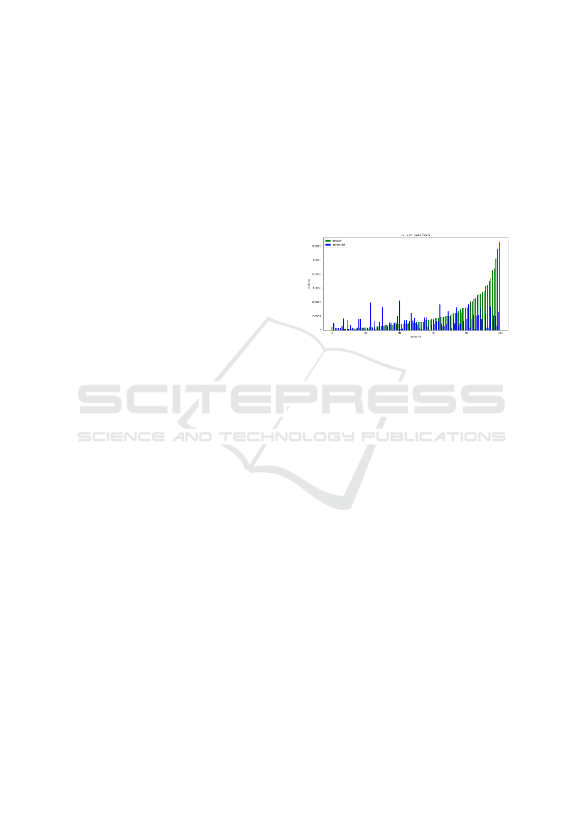
Figure 15: 100 Training instances, random, satisﬁable.

Instances used for training are from SATLIB, they

have constant number of variables, 250 before prepro-

cessing.

In Figure 15 it can be seen that tuned parameters

(blue), are faster for some of the instances but in fact

slower for those instances that can be solved very fast

with default parameters, those are instances which are

solved within single digit number of restarts.

This is probably because the model tends to

choose wider restart interval (in comparison to de-

fault’s value of 2, which is quite low), because it

was also trained on the factorization instances, which

require less frequent restarts. On those random in-

stances which take considerable time to solve by de-

fault parameters, the efﬁciency rises dramatically, and

thus tuned parameters should be used on random in-

stances which have larger number of variables, be-

cause for small instances default parameters perform

better.

This could be ﬁxed by including random instances

of different sizes in the training set, so the model

could adapt to the size of the instance better, for ex-

ample, for small instances restart frequency should be

also much smaller.

For every random unstatisﬁable instance from

training set (SATLIB) the tuned parameters are much

faster.

This plot proves that it is worth tuning solver’s

parameters in particular for unsatisﬁable instances.

There is a slight correlation between heights of green

ICAART 2022 - 14th International Conference on Agents and Artiﬁcial Intelligence

594

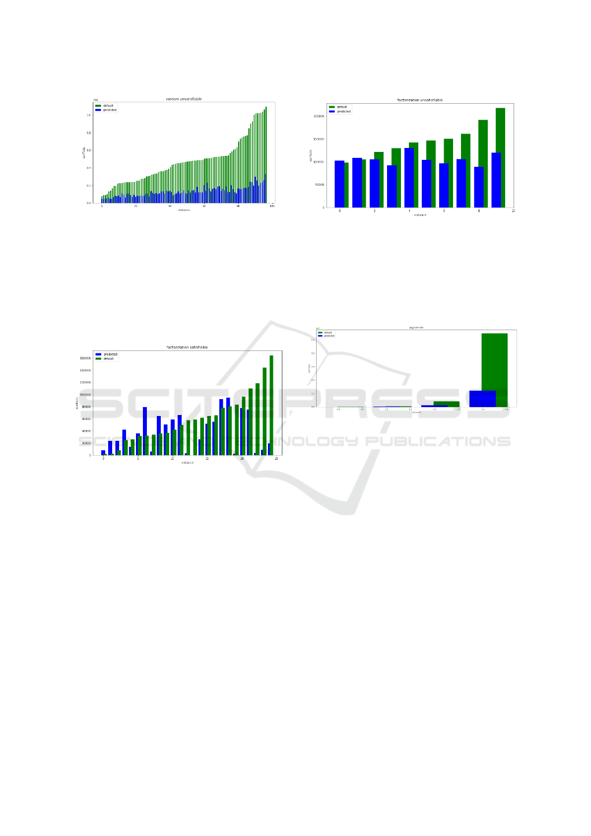
Figure 16: 97 Training instances, random, unsatisﬁable.

and blue bars on the graph, unlike for random satisﬁ-

able instances.

The hardest instances are from so called phase

transition which is a ratio of clauses to variables

around value 4.26, so roughly 4x more clauses than

variables.

The computation of features is very fast for ran-

dom instances as they have balanced ratio of clauses

and variables.

Figure 17: 25 Training instances, factorization, satisﬁable

(not prime numbers).

12/25 satisﬁable instances were actually slower

with tuned parameters but 10 of them were easy in-

stances. This may seem a bit disturbing result as ﬁrst

sight, but our hypothesis is that the cause of it, is lack

of easier instances of this type of problem in the train-

ing dataset as ﬁrst half of the plot shows. On the sec-

ond half of the graph it can be observed that for harder

instances, only two instances are slightly slower. We

would say, for harder instances these results are posi-

tive.

The model does not distinguish well between hard

and easier instances, and as a result it is predicting

restart frequency parameters similarly for both harder

and easier instances.

Another possibility can be that there is no infor-

mation to be captured from the graph structure about

how hard the instance will be.

Majority of eight out of ten instances are favoring

tuned parameters, for two easiest instances the default

Figure 18: 10 Training instances, factorization, unsatisﬁ-

able (prime numbers).

parameters perform better but only by a tiny bit of

500-1000 conﬂicts less which is small enough count

to be neglected.

The improvement is only moderate, nowhere near

the improvement observed on random unsatisﬁable

instances.

Figure 19: Training instances, pigeonhole problem.

First two bars are insigniﬁcant, but on remaining

the big improvement can be seen. Even though the

training dataset contained only these four instances

of pigeonhole problem (because higher order of this

problem is very difﬁcult and it was infeasible to per-

form grid-search on many parameters values), the

model was able to predict values correctly.

This might mean that the structure of this instance

is vastly different from all the other instances from

classes.

7.2 Performance on Testing Instances

As a testing set for random instances we generated

instances randomly but with 300 variables in compar-

ison to SATLIB’s 250, to observe whether the model

will be able to predict values correctly also for in-

stances which are much harder than the ones it was

trained on.

Plot shows very good results, so this verify my hy-

pothesis, that even model trained on smaller instances

can perform good on bigger.

For harder instances (second half of the plot),

there is only one instance which takes almost twice as

Parameter Setting in SAT Solver using Machine Learning Techniques

595

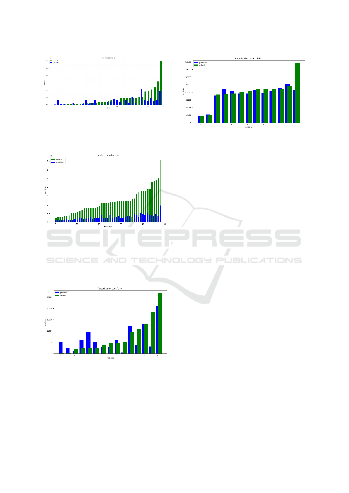
Figure 20: 36 Testing instances, random, satisﬁable.

much with tuned parameters as with the default ones.

This is probably because the structures of the ran-

dom instances are homogeneous regardless of their

size.

Figure 21: 60 Testing instances, random, unsatisﬁable.

Observed results are remarkable, all instances are

faster on tuned parameters by at least 2x, on some

instances, mostly harder ones, 3x faster.

The key takeaway is that the parameter tuning is

very effective way to improve SAT solvers perfor-

mance on unsatisﬁable instances.

Figure 22: 15 Testing instances, factorization, satisﬁable.

Similar results as on training set can be seen here

for factorization, satisﬁable instances. Performance

is better on harder instances, from harder instances

only one is outperformed by default settings. Easier

instances are solved faster by default settings, most

likely because of low base restart interval.

Figure 23: 13 Testing instances, factorization, unsatisﬁable.

For testing set we picked 2 easy instances, which

can be seen as ﬁrst 2 bars, then a few average hard

instances and one very hard, the last bar.

For easy instances there is no improvement, for

medium instances predicted parameters give steadily

100000 conﬂicts, worth noting is that, the same is for

instances in the training set. For hard instance num-

ber of conﬂicts is also close to 100000, and almost 2x

speedup can be seen. Tuned parameters perform more

less the same as default ones but we hypothesize that,

that as hardness of the instances increase the speedup

would get more signiﬁcant with it.

7.3 Planning Instances

It is unfortunate that we were unable to train the

model for planning problems. This is due to computa-

tional burden that we encountered later, in the process

of extracting features.

Constructing clause graph which is usually very

big due to the nature of planning instances and com-

puting features on it was not feasible.

If we were to start over, we would not include

clause graph for planning instances, and focus more

on graph properties of corresponding VG and VCG

graphs.

8 CONCLUSIONS

We have shown that a dependency of SAT solver’s

solving time on its parameters exists. This has been

fully illustrated in our experimental evaluation, on a

set of four, structurally diverse SAT instances.

The dependencies were measured with ﬁve of

the MiniSat’s parameters concerning heuristics and

restart policy.

The most signiﬁcant dependencies were observed

on random SAT instances exhibiting dependency on

four parameters. Except the planning instances, every

other class has shown dependency on clause decaying

ICAART 2022 - 14th International Conference on Agents and Artiﬁcial Intelligence

596

factor. Each of the studied classes were dependent on

the restart frequency.

The dependency has been utilized for automated

settings of MiniSat’s parameters using machine learn-

ing based on features extracted from graphs derived

from the input instance.

We evaluated how predicted parameters perform

on both training set and testing set.

Signiﬁcant improvement of running time has been

achieved with predicted parameters for all types of in-

stances except the planning class. The most positive

achievement was tuning parameters for unsatisﬁable

random SAT instances, where for signiﬁcant number

of instances tested we achieved up to 3x speedup.

As a suggestion for a future work, we plan to focus

on computing features of VG and VCG and leave CG

out as it is very computationally expensive and often

causes feature extractor execution time to outweigh

actual solving time.

ACKNOWLEDGEMENTS

This research has been supported by GA

CR - the

Czech Science Foundation, grant registration number

22-31346S.

REFERENCES

Sat competition website. http://www.satcompetition.org/.

Ans

otegui, C., Gir

aldez-Cru, J., and Levy, J. (2012). The

community structure of sat formulas. In Cimatti, A.

and Sebastiani, R., editors, Theory and Applications

of Satisﬁability Testing – SAT 2012, pages 410–423.

Springer.

Bennaceur, H. (2004). A comparison between sat and csp

techniques. Constraints, 9:123–138.

Biere, A., Biere, A., Heule, M., van Maaren, H., and Walsh,

T. (2009). Handbook of Satisﬁability: Volume 185

Frontiers in Artiﬁcial Intelligence and Applications.

IOS Press, NLD.

Cook, S. A. (1971). The complexity of theorem-proving

procedures. In Proceedings of the Third Annual ACM

Symposium on Theory of Computing, STOC ’71, page

151–158, New York, NY, USA. Association for Com-

puting Machinery.

Dennis, G., Chang, F. S.-H., and Jackson, D. (2006). Mod-

ular veriﬁcation of code with sat. In Proceedings of

the 2006 International Symposium on Software Test-

ing and Analysis, ISSTA ’06, page 109–120, New

York, NY, USA. Association for Computing Machin-

ery.

D’Ippolito, N., Frias, M., Galeotti, J. P., Lanzarotti, E., and

Mera, S. (2010). Alloy+hotcore: A fast approximation

to unsat core. volume 5977, pages 160–173.

en, N. and Biere, A. (2005). Effective preprocessing in sat

through variable and clause elimination. In Bacchus,

F. and Walsh, T., editors, Theory and Applications of

Satisﬁability Testing, pages 61–75. Springer.

Ganesh, V., Singh, R., Near, J., and Rinard, M. (2009).

Avatarsat: An auto-tuning boolean sat solver.

Gupta, A., Ganai, M. K., and Wang, C. (2006). Sat-

based veriﬁcation methods and applications in hard-

ware veriﬁcation. In Bernardo, M. and Cimatti, A.,

editors, Formal Methods for Hardware Veriﬁcation,

pages 108–143. Springer.

Haken, A. (1984). The Intractability of Resolution (Com-

plexity). PhD thesis, USA. AAI8422073.

Kautz, H. and Selman, B. (1992). Planning as satisﬁability.

pages 359–363.

Liang, J. H. (2018). Machine Learning for SAT Solvers.

PhD thesis, University of Waterloo.

Lourenc¸o, H., Martin, O., and St

utzle, T. (2010). Iterated

Local Search: Framework and Applications, volume

146, pages 363–397.

Marques Silva, J. P. and Sakallah, K. A. (1996). Grasp-a

new search algorithm for satisﬁability. In Proceed-

ings of International Conference on Computer Aided

Design, pages 220–227.

Mitchell, T. M. (1997). Machine Learning. McGraw-Hill.

Newsham, Z., Lindsay, W., Ganesh, V., Liang, J. H., Fis-

chmeister, S., and Czarnecki, K. (2015). Satgraf:

Visualizing the evolution of sat formula structure in

solvers. In International Conference on Theory and

Applications of Satisﬁability Testing (SAT), Austin,

USA. Springer, Springer.

Niklas E

en, N. S. (2004). Theory and applications of sat-

isﬁability testing: 6th international conference, sat,

santa margherita ligure, italy, may 5-8, 2003, se-

lected revised papers, chapter an extensible sat-solver.

Springer, pages 502–518.

Pintjuk, D. (2015). Boosting sat-solver performance on fact

instances with automatic parameter tuning.

Pipatsrisawat, K. and Darwiche, A. (2007). A lightweight

component caching scheme for satisﬁability solvers.

In Marques-Silva, J. and Sakallah, K. A., editors, The-

ory and Applications of Satisﬁability Testing – SAT

2007, pages 294–299. Springer.

Sinz, C. and Dieringer, E.-M. (2005). Dpvis – a tool to

visualize the structure of sat instances. In Bacchus,

F. and Walsh, T., editors, Theory and Applications of

Satisﬁability Testing, pages 257–268. Springer.

Soos, M., Nohl, K., and Castelluccia, C. (2009). Extend-

ing sat solvers to cryptographic problems. In Kull-

mann, O., editor, Theory and Applications of Satisﬁa-

bility Testing - SAT 2009, pages 244–257. Springer.

Xu, L., Hutter, F., Hoos, H. H., and Leyton-Brown, K.

(2008). Satzilla: Portfolio-based algorithm selection

for sat. J. Artif. Intell. Res., 32:565–606.

Parameter Setting in SAT Solver using Machine Learning Techniques

597