Exploring the Tabu Search Algorithm as a Graph Coloring Technique for

Wavelength Assignment in Optical Networks

es Gomes

, Lu

ıs Cancela

1,2

and Jo

ao Rebola

1,2

Optical Communications and Photonics Group, Instituto de Telecomunicac¸

oes, Lisboa, Portugal

Department of Science and Information Technology, Instituto Universit

ario de Lisboa (ISCTE-IUL), Lisboa, Portugal

Keywords:

Graph Coloring, Greedy, Optical Networks, Tabu Search, Wavelength Assignment.

Abstract:

The aim of this work is to study the Tabu Search algorithm as a graph coloring technique for wavelength

assignment in optical networks, a crucial function in optical network planning. The performance of the Tabu

Search is assessed in terms of the number of wavelengths and computation time and is compared with the one

of the most common Greedy algorithm. It is concluded that for real networks with a large number of nodes

and a higher variance node degree of the path graph relatively to its average node degree value, the Greedy

algorithm is preferable to the Tabu Search algorithm since it returns the same number of colors of Tabu Search,

but in a shorter computation time.

1 INTRODUCTION

Routing and Wavelength Assignment (RWA) are fun-

damental functions to transport data in an efﬁcient

way in optical networks (Winzer et al., 2018). Rout-

ing is responsible for ﬁnding the best path for a given

trafﬁc demand, and wavelength assignment (WA) is

responsible for choosing an appropriate wavelength in

that path to transport the given trafﬁc demand taking

into account the wavelength continuity and the dis-

tinct wavelength constraints (Simmons, 2014).

Several techniques have been used to solve the

WA problem, ranging from exact algorithms to

heuristics that typically give a sub-optimal solution

to the problem, but in a shorter time, like the First-

Fit or the Most Used algorithms (Simmons, 2014),

(Zangy et al., 2000). Graph coloring techniques, al-

though applied to a large range of applications, such

as constructing schedules, can also be used for WA

in optical networks (Simmons, 2014). The most used

graph coloring algorithm for WA is the Greedy algo-

rithm (Lewis, 2016). Some studies have, however,

used other Graph coloring algorithms for WA, such

as the DSATUR and RLF (Duarte et al., 2021), but

for the majority of the networks studied the Greedy

algorithm performs as well as these algorithms.

In this work we aim to study a more complex and

more rigorous graph coloring technique for WA in op-

tical networks, the Tabu Search algorithm. A perfor-

mance study is made for several network topologies in

terms of the number of colors and computation time.

Moreover, a detailed comparison with the the Greedy

algorithm is performed. The aim of these algorithms,

considering a static network scenario, is to ﬁnd the

minimum number of wavelengths that satisﬁes all the

trafﬁc demands, in a feasible and reasonable compu-

tational time.

Note that the Tabu Search algorithm is a meta-

heuristic algorithm used for solving different kinds

of problems, such as optimization problems in net-

work design (Pi

oro and Medhi, 2004). For example,

it has been used for solving RWA problems based on

Integer Linear Programing (ILP) formalisms (Wang,

2004), (Go

scie

n et al., 2014), (Dzongang et al., 2005).

Moreover, in (Hertz and Werra, 1987) this algorithm

has been used to solve graph coloring problems. But,

to the best of our knowledge, there are no works that

have used it as a graph coloring technique for WA in

optical networks, as we do in this work.

This paper is organized as follows. In Section

2, the Greedy and Tabu Search graph coloring algo-

rithms are explained and their pseudocodes and illus-

trative examples provided. In Section 3, the perfor-

mance of the Tabu Search algorithm in random graphs

and its comparison with the Greedy algorithm is stud-

ied. In Section 4, the RWA planning tool is brieﬂy

described and the performance of both algorithms as

graph coloring techniques for WA in optical networks

is assessed for several real networks. Finally, in Sec-

tion 5, the conclusions are drawn.

Gomes, I., Cancela, L. and Rebola, J.

Exploring the Tabu Search Algorithm as a Graph Coloring Technique for Wavelength Assignment in Optical Networks.

DOI: 10.5220/0010910000003121

In Proceedings of the 10th International Conference on Photonics, Optics and Laser Technology (PHOTOPTICS 2022), pages 59-68

ISBN: 978-989-758-554-8; ISSN: 2184-4364

2 GRAPH COLORING

ALGORITHMS

In this section, the Greedy and Tabu Search algo-

rithms, are explained through their respective pseu-

docode and an illustrative example is given.

2.1 Greedy Algorithm

The Greedy algorithm is probably the most used

graph coloring algorithm (Lewis, 2016). It consists

in coloring the vertices of a given graph one by one,

with some ordering strategy, so that adjacent vertices

have different colors (Lewis, 2016).

Figure 1 shows the pseudocode for Greedy algo-

rithm (Lewis, 2016). Initially S that represents the

set of colors that are going to be assigned along the

Greedy algorithm process is empty and π represents

a possible permutation of the graph vertices, e.g. de-

scending, ascending or random order of the vertices.

The for cycle in line (1) of the pseudocode goes

through the set of vertices π and, for each vertex of

π tries to ﬁnd a color class S

belonging to S to which

it can be associated. This process involves checking

the color class of the adjacent vertices. If the working

vertex is an independent set then a color S

can be as-

signed to this vertex. If this is not the case then a new

color class must be assigned (lines 7 to 9).

Figure 1: Pseudocode for Greedy algorithm.

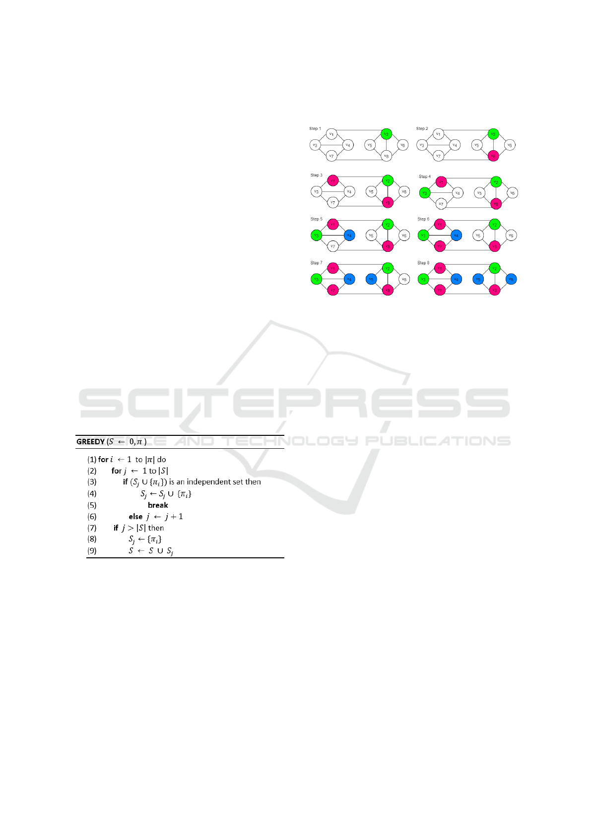
Figure 2 represents an example of the operation of

the Greedy algorithm, assuming a coloring strategy

based on the descending order of degree. The ver-

tex with the highest number of links connected, i.e.,

the highest vertex degree, is colored ﬁrst, i.e. v

step 1 is color with green (S

={green}). In step 2 the

algorithm continues the coloring with the following

highest vertex degree, v

, which is adjacent to v

it is assigned to a different color, pink (S

={pink}).

In step 3, since there are four vertices with degree 3,

one of them is randomly chosen. We have choose v

with the color class S

(step 4). This process contin-

ues until all vertices have been colored and in the end

(step8) we can see that three colors are used.

Figure 2: Greedy algorithm example.

2.2 Tabu Search Algorithm

Tabu Search is a metaheuristic algorithm, used to

solve different kinds of problems, such as graph col-

oring (Lewis, 2016). The idea of this algorithm, when

applied to graph coloring problems, is to answer the

following question: given a graph G(V,E), where V

represent the set of vertices and E the set of edges be-

tween vertices, is it possible to feasibly color it with k

colors? This algorithm has the following main steps:

1. It starts by deﬁning an initial solution S to color

the graph with a predeﬁned value k of colors,

which can be obtained randomly or by using a

constructive heuristic, like Greedy or DSATUR

(Lewis, 2016).

2. The algorithm next proceeds by computing the

number of clashes (i.e. two adjacent vertices with

the same color) which is represented by function

f(S), deﬁned by:

f (S) =

∑

∀{u,v}∈E

g(u, v) (1)

with g(u,v)=

(

1 ifc(u)=c(v),

0 otherwise.

where c(u) is the color of vertex u and c(v) is the

color of vertex v.

If g(u,v) = 1 it means that the color of the two

adjacent vertices u and v is the same and there-

fore a clash occurs. The aim of the algorithm is to

eliminate the clashes, i.e., f (S) = 0. If the num-

ber of clashes is not zero, a new solution S’ is ob-

tained, by using the neighbor operator, which is

PHOTOPTICS 2022 - 10th International Conference on Photonics, Optics and Laser Technology

deﬁned as follows: if a vertex v is assigned to a

color i, a neighbor operator corresponds to a color

change of vertex v to a new color j. Note that to

obtain this new solution S’ there are some ver-

tices color changes that can not be done. These

vertices color changes are registered in a list of

forbidden vertices color changes, called the Tabu

list T. This list is used to avoid previous unde-

sired and already checked solutions (Hertz and

Werra, 1987). If with this new solution S’ condi-

tion f (S

) < A( f (S)) is veriﬁed, the best solution

S’ is found. In this condition, A is an “aspiration

level” function that gives the possibility that so-

lutions S’ with a superior number of clashes be

chosen, with the aim to escape from local minima

(Hertz and Werra, 1987). If f (S

) = 0 and number

of operations (Niter) is less than Nmax it means

that a solution with k colors is found. If the num-

ber of operations is Nmax the algorithm stops.

3. If a solution with k colors is found the algorithm

starts again with k-1 colors.

Figure 3 shows the pseudocode of the Tabu Search

algorithm, which follows the previous explanation.

The pseudocode is initialize by deﬁning an initial so-

lution S and the Tabu list T size. While clashes occur,

i.e., f (S) > 0, a new solution S’ is searched, the con-

dition f (S

) < A( f (S)) is checked and the Tabu list T

is updated.

Figure 3: Pseudocode for Tabu Search algorithm.

If a solution with k colors ensures that the number

of clashes is zero, the algorithm tries a solution with

k−1 colors (lines 9-10). The algorithm stops when no

solution with k − 1 colors is achieved or the number

maximum of iterations is reached.

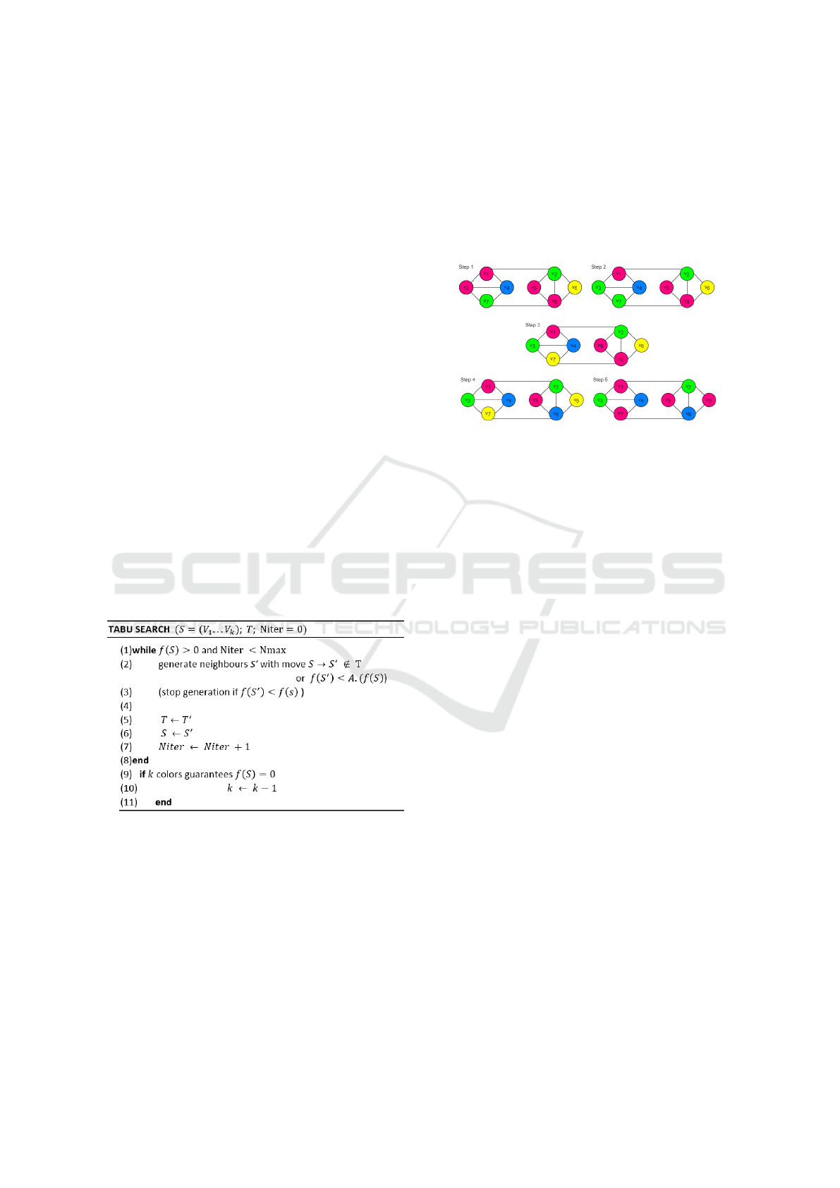
Figure 4 represents the same network of Figure

2, but now the coloring is going to be made with

the Tabu Search algorithm. The algorithm starts with

a random coloring solution (step 1). In this case,

this random solution has 4 colors and 2 clashes, so

f (S

) = 2. Once the solution has clashes, the algo-

rithm generates a new solution S’. In step 2, the neigh-

bor operator works in the vertex 3 changing the color

pink to green. This operation eliminate the clash that

occurs between vertices 1 and 3, but a new clash ap-

pears between vertices 3 and 7, keeping the number

of clashes equal to 2. The Tabu list T is updated with

this move, i.e., vertex 3 changes from pink to green.

Figure 4: Tabu Search algorithm example.

In step 3, the clash between vertices 3 and 7 is

eliminated and a better solution is found that reduces

the number of clashes to one, between adjacent ver-

tices 5 and 8. In this step, the neighbor operator works

in vertex 7, coloring it with yellow, which is one of the

four initial colors of the solution. The Tabu list T is

updated again, with the addition of the move corre-

sponding to vertex 7 colored in green. Thus, in step 3

there is a solution with 4 colors and one clash between

vertices 5 and 8.

In step 4 occurs the coloring of vertex 8 with blue.

Thus, all clashes are eliminated, i.e., f (S) = 0 and

a complete proper k coloring is found with k=4. At

this stage, the algorithm tries the solution k=3 colors.

If vertices 6 and 7 are colored with pink (step 4) or

vertices 1 and 5 are colored with yellow, this solu-

tion is feasible, with a total of k colors smaller than

initially tested, making it a better solution. Next, the

algorithm tries the solution with k=2 colors, but no

solution with proper coloring is found, so, k=3 is the

minimum number of colors.

3 PERFORMANCE OF THE TABU

SEARCH ALGORITHM IN

RANDOM GRAPHS

In this section, we study the performance of the Tabu

Search algorithm in random graphs, and compare its

performance with the one of Greedy algorithm with

descending order. We have used the implementation

of these algorithms available in (Lewis, 2016). But,

ﬁrst, we analyze the inﬂuence of the number of con-

straint checks (Lewis, 2016) on the accuracy of the

Exploring the Tabu Search Algorithm as a Graph Coloring Technique for Wavelength Assignment in Optical Networks

Tabu Search algorithm, in order to minimize the re-

spective computation time.

Random graphs, G

n,p

, are graphs with n ver-

tices characterized by the parameter p, which corre-

sponds to the probability of two vertices being adja-

cent (Lewis, 2016). The parameter p can be given by

p =

∑

i=1

n−1

(2)

where Dg

is the degree of vertex i and n is the number

of vertices.

Random graphs are built by generating random

matrices with a n × n dimension according to the pa-

rameter p. Each matrix position represents a pair of

vertices; if its value is one it means that the vertices

are adjacent, if its value is zero, the vertices are non-

adjacent. These values are randomly generated using

a uniform distribution. In particular, when p = 1, it

means that the degree of any vertex of the matrix is

n − 1, i.e., all vertices of the matrix are adjacent to

each other.

3.1 Inﬂuence of the Number of

Constraint Checks

In order to compute the time needed for the Tabu

Search algorithm to provide a graph coloring solution,

we ﬁrst analyze the minimum number of constraint

checks needed to achieve the best solution. Constraint

checks are the operations within the Tabu Search al-

gorithm that involve information requests about the

graph, such as determining the degree of a vertex, or

determining if two vertices are adjacent or not (Lewis,

2016).

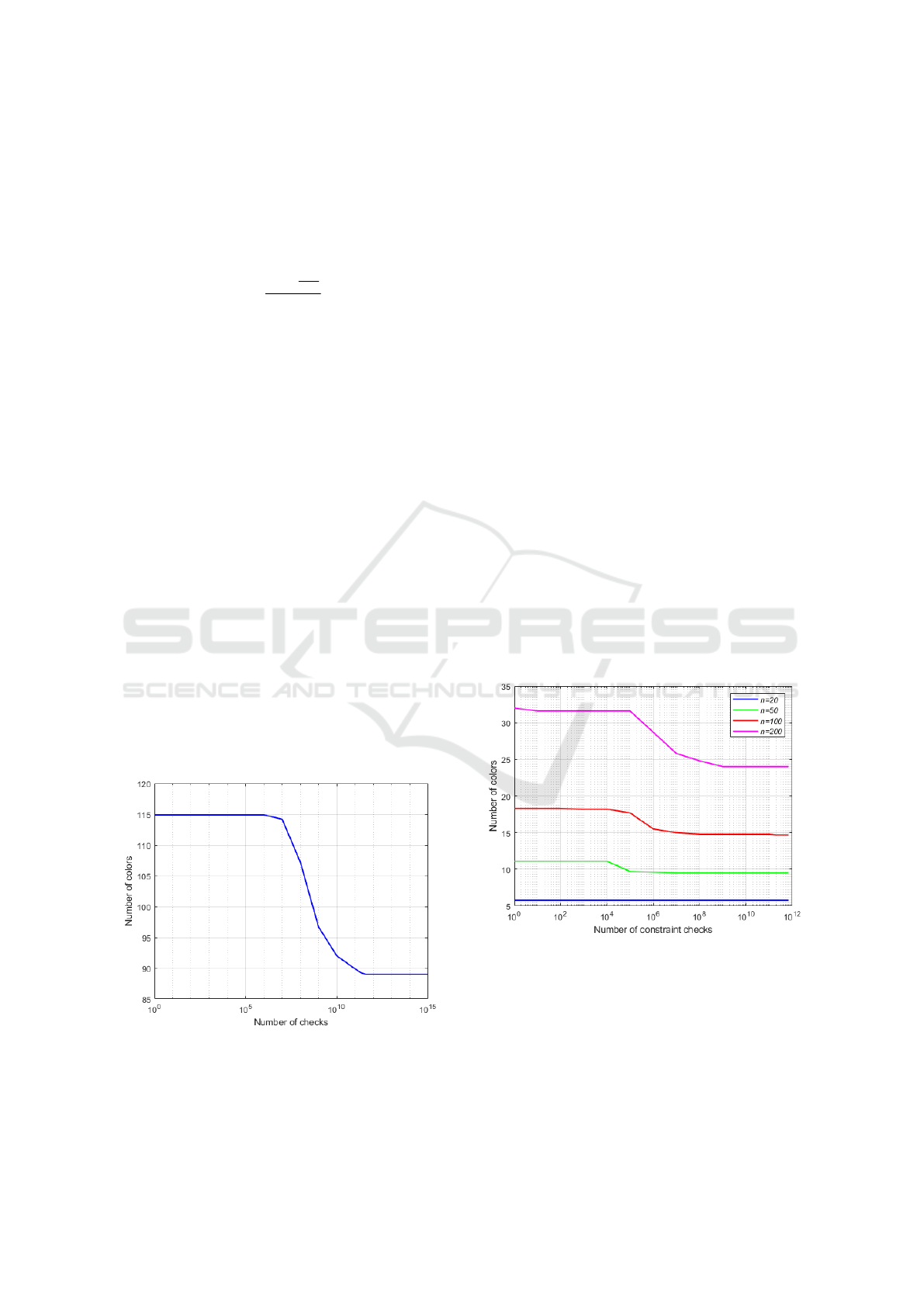
Figure 5: Number of colors as a function of the number of

constraint checks considering the Tabu Search algorithm for

n = 1000 and p = 0.5.

In Figure 5, the number of colors as a function

of the number of constraint checks is represented for

n = 1000 and p = 0.5, considering the generation

of 10 random graphs for each number of constraint

checks. As can be observed, the number of colors is

minimized only when the number of checks is above

1 × 10

. From that point on, the number of colors

remains practically constant. Thus, for n = 1000, a

number of constraint checks of 4 × 10

is sufﬁcient

to ensure that the optimal solution is reached. It was

conﬁrmed that the parameter p does not inﬂuence the

number of constraint checks required to achieve the

minimum number of colors with the Tabu Search.

This number only depends on the size of the graph.

Figure 6 shows the evolution of the number of

colors for Tabu Search algorithm as the number of

constraint checks increases for n = 20, 50, 100 and

200 and p = 0.5. The number of constraint checks

in this study is between 1 and 1 × 10

. From Fig-

ure 6, it can be concluded that for n = 20, only one

constraint check is needed to obtain the best solution.

Likewise for n = 50, n = 100 and n = 200, a num-

ber of constraint checks above, respectively, 1 × 10

1 × 10

and 1 × 10

is needed to obtain the best so-

lution. Below these values of constraint checks, the

required number of colors increases with the graph

size, as expected. In what concerns to the compu-

tational effort, as n decreases, the required number of

constraint checks that minimizes the number of colors

also decreases, and therefore the computation time for

lower n will be lower as well.

Figure 6: Number of colors as a function of the number

of constraint checks imposed on Tabu Search for p = 0.5

considering different values of n.

The study of the number of constraint checks

needed by the Tabu Search algorithm to minimize the

number of colors for each graph was carried out to

save computation time and is shown in Figure 7. The

number of constraint checks, as observed in Figure

7 for the Tabu Search curve, depends remarkably on

the number of vertices, n, in the graph. This study

PHOTOPTICS 2022 - 10th International Conference on Photonics, Optics and Laser Technology

has been performed considering 25 simulations for a

parameter p = 0.5. However, from extensive simu-

lation results, it has been concluded that there is no

dependence between the number of constraint checks

required and the parameter p. Thus, regardless the

value of p, from Figure 7, it is possible to obtain an

approximation for the required number of constraint

checks for any number of vertices n that minimizes

the number of colors in a random graph. To obtain

such approximation in Figure 7, a curve ﬁtting has

been performed relatively to the Tabu Search curve,

including linear, quadratic, cubic and fourth degree

ﬁttings. Note that for proper ﬁtting, the logarithm

base 10 of the number of checks has been used.

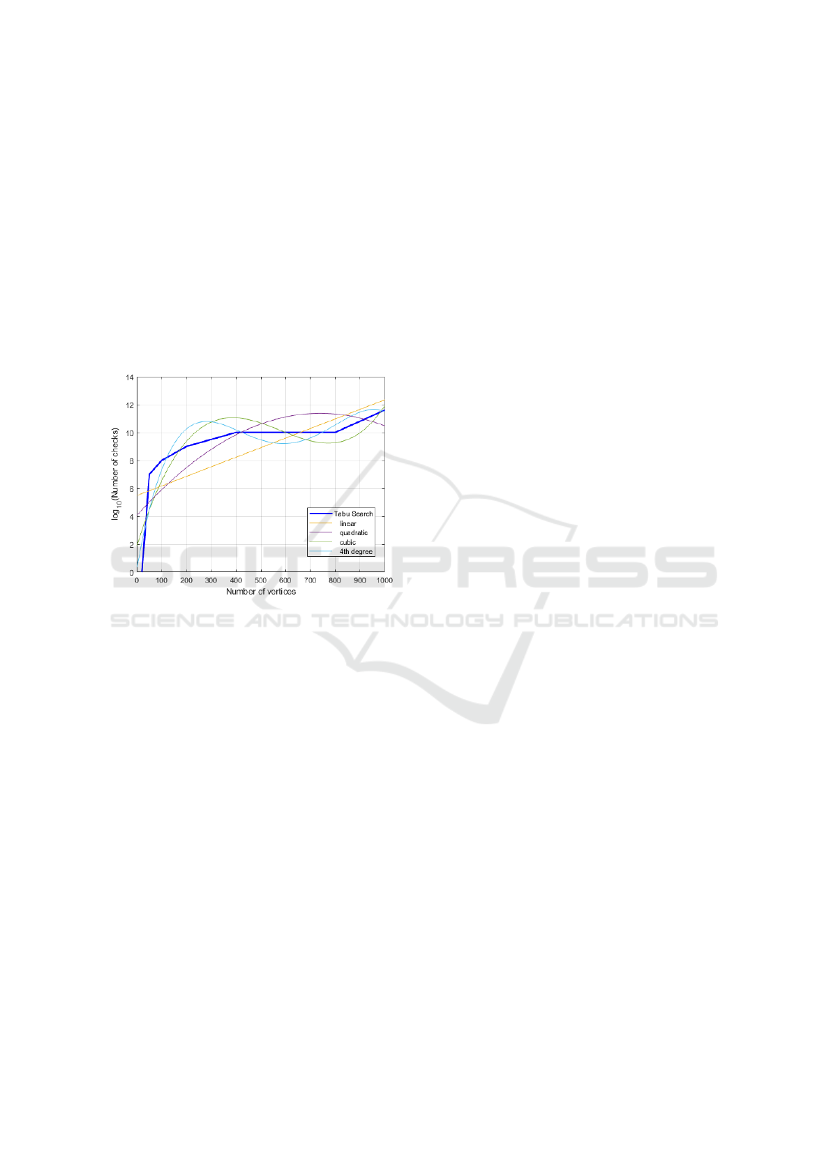
Figure 7: Number of constraint checks as function of the

number of vertices and some ﬁtting curves.

As can be observed in Figure 7, the linear and

quadratic ﬁttings, respectively, below n = 500 and

n = 300, predict a number of checks much smaller

than the one given by the Tabu Search. The cubic and

fourth degree ﬁttings predict a very similar number

of constraint checks, but we prefer to use the cubic

ﬁtting, because it represents a simpler function. The

cubic ﬁtting is given by:

6.4×10

−8

−1.1×10

−4

+5.7×10

−2

n+1.9 (3)

3.2 Comparison with the Greedy

Algorithm

After studying the appropriate number of constraint

checks to use in the Tabu Search algorithm, the per-

formance of the Greedy and Tabu Search algorithms

in ﬁnding the optimal color solution is also studied

and compared considering random graphs.

Figure 8 a) shows the number of colors as a func-

tion of p for n = 1000 calculated using the Greedy

(with random and descending order) and the Tabu

Search algorithms. A very good agreement between

the Tabu Search results and the ones presented in Fig-

ure 4.6 of (Lewis, 2016) is found. It can be observed

from Figure 8 a) that for p = 0 and p = 1, there are

no difference between the algorithms in the number

of colors, as these are the cases where no adjacency

and full adjacency between vertices occur, respec-

tively. That is, if the vertices are all non-adjacent,

the same color, independently of the algorithm, can

be applied to all vertices. Similarly, if all vertices are

adjacent between each other, then each vertex is as-

signed its own color. Also from Figure 8 a), we can

observe that the Tabu Search needs fewer colors than

the Greedy algorithm, and that the difference in the

number of colors increases with p, but the relative

percentage increase is always around 40%. For ex-

ample, for p = 0.1, the Tabu Search gives 21 colors

and the Greedy 30 colors, which is an increase of 9

colors (43 % increase); for p = 0.5, the Tabu Search

provides 89 colors and the Greedy gives 125 colors,

which is an increase of 36 colors (40 % increase) and

for p = 0.9, the Tabu Search gives 229 colors and the

Greedy gives 313 colors, which is an increase of 84

colors (37 % increase). Although in Figure 8 a) the

results obtained with Greedy random and Greedy de-

scending orders seem to be very similar, in the inset

of Figure 8 a), it can be seen that the descending order

gives always slightly better results (1 color difference)

(Duarte, 2020).

Figures 8 b) and c) shows again the performance

of both Greedy and Tabu Search algorithms for ran-

dom graphs, but for 100 and 20 vertices, respectively,

as a function of p. As observed in Figures 8 b) and

c), it can be concluded that the Tabu Search per-

forms once again better than the Greedy algorithm by

predicting less colors and this behavior is more pro-

nounced for increasing values of n and p.

To better understand the conclusions presented in

Figure 8, Figure 9 shows the increase in percentage

of the number of colors as a function of p predicted

by the Greedy algorithm in comparison with the Tabu

Search, considering n = 20, 50, 100, 200, 1000. Note

that 25 simulations were performed to obtain the re-

sults presented.

From Figure 9, it can be concluded that the greater

the number of vertices in the graph, the greater the

percentage growth. The maximum value found is

around 40%. For p = 0.1 and n = 200, there is a max-

imum 40% increase in the number of colors used by

the Greedy algorithm in comparison with the number

of colors predicted by the Tabu Search, whereas, for

n = 100, there is only 32% increase, for n = 50, there

is 10% increase and, for n = 20, there is only 3% in-

crease. From these results, it can be concluded that

Exploring the Tabu Search Algorithm as a Graph Coloring Technique for Wavelength Assignment in Optical Networks

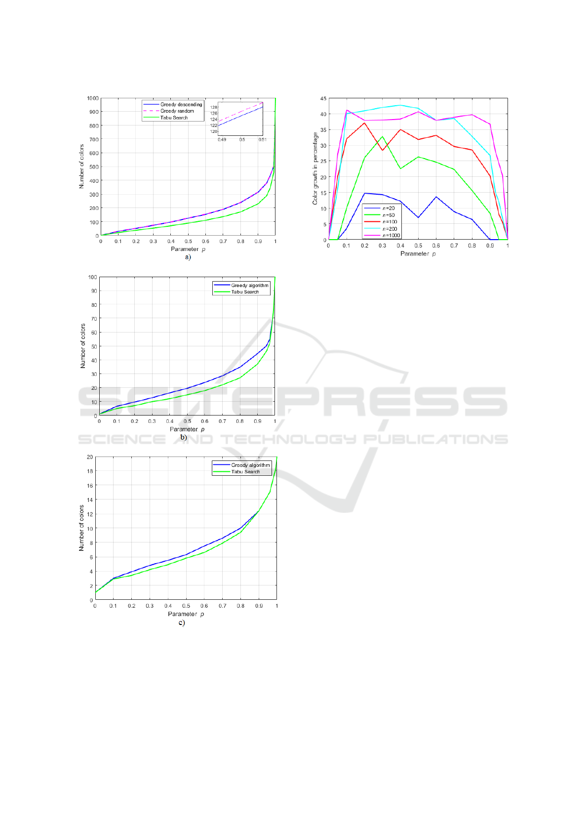
Figure 8: Number of colors as a function of p calculated

using the Greedy and Tabu Search algorithms for random

graphs for a) n = 1000, b) n = 100 and c) n = 20.

the decrease in the total number of colors attributed

by the Tabu Search in comparison with the Greedy is

more pronounced in graphs with more vertices.

Figure 9: Percentage of the number of colors increase be-

tween Tabu Search and Greedy algorithms for n = 20, n =

50, n = 100, n = 200 and n = 1000 as a function of p.

4 TABU SEARCH ALGORITHM

AS A GRAPH COLORING WA

TECHNIQUE

In this section, we assess the performance of the Tabu

Search algorithm as a graph coloring WA technique in

several real networks. A comparison with the Greedy

algorithm is also performed. But, ﬁrst, we brieﬂy out-

line the RWA planning tool used, as well as, the net-

work physical and logical topologies studied.

4.1 RWA Planning Tool

The planning tool used to solve the RWA problem

was developed in (Duarte, 2020) and extended in this

work in order to study the performance of the Tabu

Search algorithm as a graph coloring WA technique.

The planning tool has the following three main func-

tionalities:

1. Deﬁnition of the physical and logical topologies

characterized, respectively, by the adjacency and

the trafﬁc matrices.

2. Routing algorithm based on the Yen’s k-shortest

path algorithm.

3. WA algorithms based on graph coloring tech-

niques: Greedy and Tabu Search algorithms. Note

that before using the Graph Coloring algorithms,

the path graph G(W, P) must be computed. This

graph is obtained from the graph G(V, E) that rep-

resents the physical topology. The vertices of

G(W, P) represent the optical paths and P rep-

resents the set of links between those vertices

(Duarte, 2020). These links are between one or

PHOTOPTICS 2022 - 10th International Conference on Photonics, Optics and Laser Technology

more vertices (i.e. paths) that share one or more

physical links. After obtaining the graph G(W, P),

the vertices can be colored considering the Greedy

and the Tabu Search algorithm explained in Sec-

tion 2. The number of colors obtained corre-

sponds to number of wavelengths needed for solv-

ing the RWA problem.

4.2 Parameters of the Network Physical,

Logical and Path Topologies

The network physical topologies used in this work

are the COST239 (Niksirat et al., 2016), NSFNET

(LaQuey, 1990), UBN (Biernacka et al., 2017) and

CONUS with 30 nodes (Monarch Network Archi-

tects, 1999), which we denominate in this work as real

networks.

A network physical topology can be characterized

by several parameters such as the average node degree

and the variance node degree, respectively, given by

(Fenger et al., 2000):

d =

∑

i=1

(4)

∑

i=1

(Dg

− d)

n − 1

(5)

Table 1: Real networks physical topology parameters.

Average Variance

Network Nodes Links Node Node

Degree Degree

COST239 11 26 4.7 0.4

NSFNET 14 21 3.0 0.3

UBN 24 43 3.6 0.9

CONUS 30 36 2.4 0.4

Table 1 shows the information regarding the net-

work physical topologies with respect to the number

of nodes and links, average and variance of the node

degree. The variance node degree helps to understand

how regular the network is from the point of view

of the number of links at each node in the network

(Fenger et al., 2000). Higher variances correspond

to more irregular networks. When the variance node

degree is zero, it means that all nodes have the same

number of links (Fenger et al., 2000).

The parameters used to characterize the physical

topology, i.e. the average and variance node degree,

can also be used to characterize the logical topology.

Table 2 presents these parameters considering that a

full mesh logical topology is applied over the physi-

cal topologies. In this scenario, the average node de-

gree is N − 1. Furthermore, the variance node degree

is zero, because all nodes have the same number of

links. In table 2 the number of bidirectional paths for

a full mesh logical topology is also shown and is given

n(n−1)

Table 2: Real networks logical topology parameters.

Number of Average Variance

Network Paths node node

degree degree

COST239 55 10 0

NSFNET 91 13 0

UBN 276 23 0

CONUS 435 29 0

Also, the average and variance node degree pa-

rameters can be evaluated in the context of the path

graph G(W, P), as shown in Table 3. The parameter

p is also presented in Table 3. A high average value

means that on average, one or more links of every path

are being used by several different paths. From Table

3 it can be observed that the variance node degree is at

least one order of magnitude higher than the average

node degree. This means that there are some links

belonging to a path (i.e. vertex) that are being used

by many other different paths, and also that there are

some links belonging to a path that are not being used,

or are slightly used by other paths. So, networks with

high path variances need a high number of colors, as

we will discuss in subsection 4.3.

Table 3: Real networks path topology parameters.

Para- Average Variance

Network meter Node Node

p Degree Degree

COST239 0.101 5.6 14

NSFNET 0.25 22.5 121

UBN 0.2250 61.9 1.2840 × 10

CONUS 0.379 164.6 4.3696 × 10

4.3 Performance Analysis

In this subsection, the performance of Greedy and

Tabu Search algorithms are assessed and compared

when applied to the real networks described in sub-

section 4.2.

Table 4 presents the number of colors and the

corresponding simulation times for the networks

COST239, NSFNET, UBN and CONUS with 30

nodes, considering a full mesh logical topology, ob-

tained with the Greedy and Tabu Search algorithms.

From the results presented in Table 4, regarding

the simulation time, it is observed that the Greedy al-

gorithm is 4 times faster than the Tabu Search for the

COST239 network and almost 10 times faster than

the Tabu Search for the CONUS network. Thus, the

Exploring the Tabu Search Algorithm as a Graph Coloring Technique for Wavelength Assignment in Optical Networks

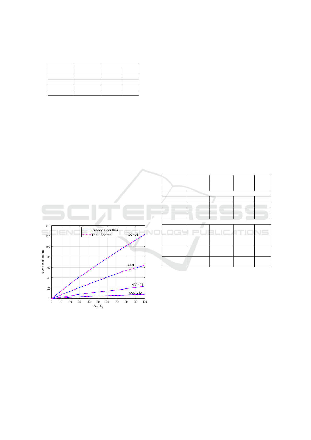
Table 4: Number of colors and simulation time obtained by

Greedy and Tabu Search for some networks.

Network Number of Time (sec)

colors Greedy Tabu

COST239 8 0.002 0.008

NSFNET 24 0.009 0.015

UBN 64 0.014 0096

CONUS 123 0.040 0.373

Greedy algorithm leads to a faster simulation time

than the one obtained with the Tabu Search.

Also, as observed in Table 4, the number of colors

obtained with the Greedy and Tabu Search algorithms

for the networks considered is the same. However, in

section 3, considering random graphs, we have seen

that the Tabu Search predicts a lower number of col-

ors than the Greedy algorithm. In order to understand

this apparently contradicting behavior, in the follow-

ing, we are going to study the inﬂuence of the trafﬁc

pattern in the number of colors obtained by the two

algorithms. Therefore, we are going to change the

trafﬁc matrix in order to obtain various logical topolo-

gies different from the full mesh topology considered

for the networks presented in Table 4. First, we de-

ﬁne a metric called the percentage of network trafﬁc,

denoted as N

. This metric ranges from 0 (no net-

work trafﬁc) to 100% (full mesh topology) and aims

to quantify the change of network trafﬁc in a trafﬁc

matrix for different networks.

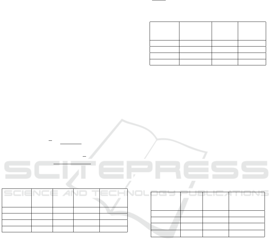
Figure 10: Number of colors provided by the Greedy and

Tabu Search algorithms for some networks as function of

Figure 10 shows the number of colors as a func-

tion of the percentage of network trafﬁc N

, for the

networks considered in Table 4, using the Greedy and

Tabu Search algorithms. From Figure 10, it can be

observed that, when N

= 0, as there is no trafﬁc in

the network, no colors are assigned. When N

> 0,

the two algorithms give exactly the same number of

colors. Thus, it can be concluded that the change of

the trafﬁc matrix (i.e. the logical topology) does not

produce any differences on the number of colors pre-

dicted by both algorithms. The reason for this be-

havior is going to be detailed next, but relies on the

fact that the variance node degree of the path matrix

is considerably greater than the corresponding aver-

age value.

Next, we are going to investigate the impact of the

average and variance node degrees of the path graph

G(W, P) in the performance of the Greedy and Tabu

Search algorithms, in order to try to explain why the

two algorithms give the same number of colors when

real networks are considered, independently of the

network trafﬁc, and different number of colors with

random graphs.

Table 5: Average and variance node degree and number of

colors given by the Greedy with descending order and Tabu

Search algorithms for real networks and for random path

graphs with the same characteristics, n and p, of the real

networks.

Average Variance Greedy Tabu

Network node node des- Sear

degree degree cend ch

Real networks

COST239 5.6 14 8 8

NSFNET 22.5 121 24 24

UBN 61.9 1.3 × 10

64 64

CONUS 164.6 4.4 × 10

123 123

Random path graphs with uniform distribution

n = 55

5.88 5.88 4.6 5

p = 0.1

n = 91

22.5 14 11 8

p = 0.25

n = 276

61.9 51.9 21 15

p = 0.225

n = 435

170.2 164.5 47 34

p = 0.392

In Table 5, the average and the variance node de-

grees of the path graph, G(W, P) of the COST239

(n = 55 and p = 0.101), NSFNET (n = 91 and p =

0.25), UBN (n = 276 and p = 0.225) and CONUS

with 30 nodes (n = 435 and p = 0.392) networks

and the respective number of colors predicted by the

Greedy and Tabu Search algorithms are presented for

a full mesh logical topology, i.e. N

= 100%. The

same network parameters are also presented for ran-

dom graphs (where the corresponding path matrix is

generated with a uniform distribution), with the same

number of paths and parameter p of the referred net-

works.

As can be observed in Table 5, the average node

degree of the path graph in real networks and random

graphs is very similar as it depends on the number of

paths and on the parameter p that is the same for the

real and random networks. However, it can be no-

PHOTOPTICS 2022 - 10th International Conference on Photonics, Optics and Laser Technology

ticed that in random graphs, the variance node degree

has a similar magnitude relatively to the average node

degree, while, in real networks, the variance node de-

gree is at least one order of magnitude higher than

the average node degree. The lower variance found

in random graphs is due to the uniform distribution

of 1’s in the path matrix, that deﬁnes the graph path

G(W, P) (e.g. for p = 0.1 it means that each line of

the matrix has 10% of ones and 90% of zeros on av-

erage), while the higher variances found in real net-

works are due to the non-uniform distribution of 1’s

in the path matrix. Furthermore, in random graphs,

for lower variance node degrees, the difference in col-

ors between Greedy and Tabu Search is notorious,

whereas in real networks both algorithms produce the

same number of colors. For example, for n = 435 and

p = 0.392, in Table 5, the variance node degree for

the CONUS with 30 nodes network is 4370, whereas

for the respective random graph, the variance has a

much lower value, 164.5. So, this ﬁnding can jus-

tify the fact that the number of colors computed by

the Greedy and Tabu Search algorithms when random

graphs are used is different, while the same number of

colors is obtained when real networks are considered.

To further conﬁrm this ﬁnding we are going to

study the evolution of the number of colors as a func-

tion of the variance node degree of the path graph,

G(W, P), for both Greedy and Tabu Search algo-

rithms.

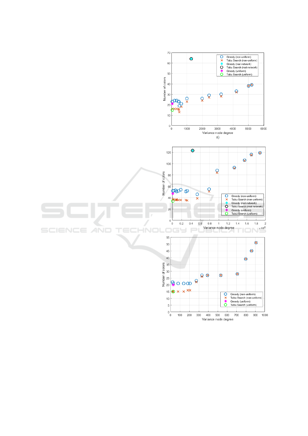
Figure 11 shows the number of colors obtained

with the Greedy and Tabu Search algorithms as a

function of the variance node degree for random ma-

trices using uniform and non-uniform distributions

with the same number of paths n and parameter p of

the real networks: a) UBN and b) CONUS with 30

nodes. In Figure 11 c), the case of the random graph

with n = 100 and p = 0.5 is also studied considering

uniform and non-uniform distributions. In Figures 11

a) and b), we also represent the number of colors cor-

responding to the real cases of UBN and CONUS with

30 nodes network, respectively.

As can be seen in Figure 11, for higher vari-

ance node degrees, the number of colors given by

Greedy and Tabu Search algorithms tends to con-

verge, whereas for lower variances the number of col-

ors produced by these algorithms is different, with

Tabu Search algorithm presenting a lower number of

colors. This behavior is observed for all the three net-

works studied. For example, in Figure 11 c), for a

low variance value of around 27, the Greedy algo-

rithm produces, respectively, 22 and 20 colors, with a

non-uniform and a uniform distribution, whereas the

Tabu Search produces 15 colors for both distributions.

Likewise, in Figure 11 c), for a high variance value of

Figure 11: Number of colors obtained with the Greedy and

Tabu Search algorithms for random graphs as a function of

the variance node degree for a) n = 276 and p = 0.225, b)

n = 435 and p = 0.392 and c) n = 100 and p = 0.5.

900, both algorithms produce around 52 colors with a

non-uniform distribution. In Figures 11 a) and b), the

number of colors obtained in the UBN and CONUS

with 30 nodes networks is also represented for both

Exploring the Tabu Search Algorithm as a Graph Coloring Technique for Wavelength Assignment in Optical Networks

algorithms. It can be observed that in these scenarios,

there are no difference between the number of colors

given by the Tabu Search and the Greedy algorithms,

which can be explained by the higher variances val-

ues relatively to its average values and also due to the

higher number of colors used. In the limit, when the

maximum number of colors is used both algorithms

must return the same number of colors.

5 CONCLUSIONS

In this work, the performance of a metaheuristic al-

gorithm, the Tabu Search algorithm, has been studied

as a graph coloring technique for WA in optical net-

works, as well as in randomly generated path graphs

and his performance has been compared with the one

of the Greedy algorithm.

The Tabu Search algorithm, when the path graph

is obtained randomly (with a uniform distribution) has

been shown to have a superior performance to the

Greedy algorithm. In particular, when n = 1000 and

p = 0.5, the Tabu Search algorithm returns only 89

colors, whereas the Greedy algorithm gives 124 col-

ors, which represents a decrease of 35 colors. How-

ever, when real networks are considered, both Greedy

and Tabu Search algorithms give the same number of

colors. We have found that as the variance node de-

gree of the path graph, G(W, P), increases the Greedy

and Tabu Search algorithms tend to return the same

number of colors, whereas when the variance gets

lower this number of colors becomes different. So,

we can conclude that in real network scenarios the

simplest and faster Greedy algorithm sorted with de-

scending order should be used, instead of the more

complex and slower Tabu Search algorithm, since real

networks have typically high variance node degree

values which causes the Tabu Search and Greedy al-

gorithms to have a similar performance.

ACKNOWLEDGEMENTS

This work was supported under the project of Instituto

de Telecomunicac

oes UIDB/50008/2020.

REFERENCES

Biernacka, E., Domzal, J., and W

ojcik, R. (2017). In-

vestigation of dynamic routing and spectrum allo-

cation methods in elastic optical networks. Inter-

national Journal of Electronics and Telecommunica-

tions, 63:85–92.

Duarte, I. (2020). Exploring graph coloring heuristics for

optical networks planning. Master’s thesis, ISCTE -

Instituto Universit

ario de Lisboa.

Duarte, I., Cancela, L., and Rebola, J. (2021). Graph color-

ing heuristics for optical networks planning. In Tele-

coms Conference (ConfTELE), pages 1–6.

Dzongang, C., Galinier, P., and Pierre, S. (2005). A tabu

search heuristic for the routing and wavelength assign-

ment problem in optical networks. IEEE Communica-

tions Letters, 9(5):426–428.

Fenger, C., Limal, E., and Gliese, U. (2000). Statistical

study of the inﬂuence of topology on wavelength us-

age in WDM networks. In Optical Fiber Communi-

cation Conference, pages 171–173. Optical Society of

America.

scie

n, R., Klinkowski, M., and Walkowiak, K. (2014). A

tabu search algorithm for routing and spectrum alloca-

tion in elastic optical networks. In 16th International

Conference on Transparent Optical Networks (ICTON

2014).

Hertz, A. and Werra, D. (1987). Using tabu search tech-

niques for graph coloring. Computing, 39:345–351.

LaQuey, T. (1990). NSFNET. In The User’s Directory of

Computer Networks, pages 247–250, Boston. Digital

Press.

Lewis, R. (2016). A Guide to Graph Coloring: Algorithm

and Applications. Springer, Switzerland.

Monarch Network Architects (1999). CONUS WDM net-

work topology. http://monarchna.com/topology.html.

Niksirat, M., Hashemi, S. M., and Ghatee, M. (2016).

Branch-and-price algorithm for fuzzy integer pro-

gramming problems with block angular structure.

Fuzzy Sets and Systems, 296:70–96.

oro, M. and Medhi, D. (2004). Routing, Flow, and Ca-

pacity Design in Communication and Computer Net-

works. MORGAN KAUFMANN PUBLISHERS.

Simmons, J. (2014). Optical Network Design and Planning.

Springer, New York, USA, 2nd edition.

Wang, S. (2004). A tabu search heuristic for routing in

WDM networks. Master’s thesis, University of Wind-

sor.

Winzer, P. et al. (2018). Fiber-optic transmission and net-

working: the previous 20 and the next 20 years. Optics

Express, 26(18):24190–24239.

Zangy, H., Juez, J., and Mukherjeey, B. (2000). A review

of routing and wavelength assignment approaches for

wavelength-routed optical WDM networks. Optical

Networks Magazine, 1:47–60.

PHOTOPTICS 2022 - 10th International Conference on Photonics, Optics and Laser Technology