Classification of Brain Tumour Tissues in Human Patients using

Machine Learning

Françoise Bouvet

, Hussein Mehidine

, Bertrand Devaux

2,3,4

, Pascale Varlet

2,5,6

and Darine Abi Haidar

1,7,*

Université Paris-Saclay, CNRS/IN2P3, IJCLab, 91405 Orsay, France

Université de Paris, Faculté de Médecine Paris Descartes, 75006 Paris, France

Service de Neurochirurgie, Hôpital Lariboisière, 75010 Paris, France

Pôle Neurosciences, GHU-Paris, 75014 Paris, France

Department of Neuropathology, GHU Paris-Psychiatrie et Neurosciences, Sainte-Anne Hospital, Paris, France

IMA BRAIN, INSERM U894, Centre de Psychiatrie et de Neurosciences, F-75014 Paris, France

Université de Paris, IJCLab, 91405 Orsay, France

Keywords: Classification, Endogenous Fluorescence, Machine Learning, Decision Trees.

Abstract: Delineating brain tumor margins as accurately as possible is a challenge faced by the neurosurgeon during

tumor resections. The extent of resection is correlated with the survival rate of the patient while preserving

healthy surrounding tissues is necessary. Real-time analysis of the endogenous fluorescence signal of brain

tissues is a promising technique to answer this problem. Multimodal optical analysis has been proved to be a

powerful tool to discriminate tumor samples of different grade of gliomas and meningiomas from healthy

control samples. In this study, Machine Learning methods are evaluated to improve the accuracy of such

discrimination. Each sample is described by 16 feature given in input to a Decision Tree based model. Once

the learning step is completed, the classifier achieves a 95% correct classification on unknown samples. This

study shows the potential of Machine Learning to discriminate between tumoral and non tumoral tissues based

on optical parameters.

1 INTRODUCTION

Brain and central nervous system cancer is one of the

most lethal cancers that affect humans (Buckner,

2007). Many types of brain tumors exist, which are

classified into different categories and grade

according to their originating cells and pathological

class (Louis, 2016).

Nowadays, total resection is still the primary

therapy for treating the majority of brain tumours and

is considered as the most critical stage in the therapy

procedure of these tumors. The main challenge of the

neurosurgical operations is to obtain a precise

identification of the margins of the tumor in order to

achieve a complete resection (Wilson, 2014). These

margins often contain diffuse isolated tumor cells

outside the solid area that have a visual appearance

similar to adjacent healthy areas, making the surgeon

unable to correctly identify these margins. The

inability to fully visualize these limits results in

corresponding author: darine.abihaidar@ijclab.in2p3.fr

incomplete surgical resection, which increases the

risk of recurrence. Similarly, unnecessary removal of

healthy brain tissue that does not contain tumor cells

can lead to major neurological deficits that affect the

patient’s quality of life.

Therefore, and in order to improve diagnosis

information on these margins and to confirm the

success of the operation, biopsy samples are extracted

from these areas for histological analysis, which

involves Haematoxylin and Eosin (H&E) staining,

but the results of this post-operative analysis are

provided a few days later and this information is not

available for the surgeon during surgery.

However, several techniques have been proposed,

developed and transferred to the operation room to

address this problem such as intraoperative-MRI and

ultrasound imaging (Kubben, 2011) (Unsgaard,

2006). The aim of these techniques is to help the

surgeon properly define the limits of the tumor and to

precise spatial information on tumor infiltration at the

Bouvet, F., Mehidine, H., Devaux, B., Varlet, P. and Haidar, D.

Classiﬁcation of Brain Tumour Tissues in Human Patients using Machine Learning.

DOI: 10.5220/0010909700003121

In Proceedings of the 10th International Conference on Photonics, Optics and Laser Technology (PHOTOPTICS 2022), pages 53-58

ISBN: 978-989-758-554-8; ISSN: 2184-4364

cellular scale. However, the information provided by

these techniques have not reached the reliability of

the gold-standard histological post-surgery analysis.

To address this challenge, our team at the IJCLab

laboratory is developing a new intraoperative optical

tool that aims to diagnose tumor zones at the cellular

scale in order to obtain fast and accurate information

on the tissue’s nature. This tool consists of a

miniature non-linear multimodal endomicroscope.

This endomicroscope is able to detect both the

quantitative (fluorescence lifetime measurement and

spectral measurement) and qualitative (fluorescence

imaging) response of endogenous fluorescence under

two-photon excitation (TPE) and the detection of the

generation of the second harmonic (SHG) (Ibrahim,

2016) (Sibai, 2018).

However, the development of this tool requires in

parallel the construction of a tissue database that

includes the different imaging modalities that we

want to integrate into our endomicroscope. The

purpose of this database is to characterize and to

discriminate different types of brain tissues, whether

healthy or tumoral, through their specific optical

signatures. Different analysis methods and data

processing will be developed and implemented in our

endomicroscope. The final aim is, based on this

database, to be able to provide the surgeon a fast,

reliable and accurate diagnosis in real time.

In our previous studies, and through different

quantitative optical parameters, we managed to

discriminate, with high specificity and sensitivity,

healthy human brain tissues, from secondary and

primary brain tumors (Poulon, 2018)(Poulon, 2018)

low and high grade glioma (Mehidine, 2019), and

grade I and grade II meningioma (Mehidine, 2021).

The aim of this study is to expand our analysis

towards using Machine Learning (ML) methods to

discriminate healthy from tumor tissues using these

quantitative parameters. ML approach allows to

combine several optical parameters thus combining

the information provided by the different endogenous

fluorescence molecules. As the histological

classification was known, we were able to investigate

supervised methods. Decision Tree is commonly used

for classification and has the benefit of being among

the most explainable ML models. Two studies are

presented, one in the visible excitation domain using

375 and 405 nm, and one in the Deep Ultra-Violet

(DUV) using 275 nm.

2 MATERIALS AND METHODS

2.1 Samples

Samples were obtained from the department of

neurosurgery of Sainte Anne Hospital (Paris) upon

the approval of the Sainte-Anne Hospital – University

Paris Descartes Review Board (CPP Ile de France 3,

S.C.3227). All methods and measurements were

carried out in accordance with the relevant guidelines

and regulations of the cited approval. Informed

consents were obtained also from all patients included

in this study. Each obtained sample was directly sent

after the surgery in a saline solution towards the

neuropathology department in Saint-Anne Hospital

where the visible measurement setup is located. More

details about the Visible measurement setup were

published elsewhere (Poulon, 2017)(Zanello,

2017)(Mehidine, 2018). Afterwards, each collected

sample was stored at −80 °C. Few hours before

cutting, the sample were put at −20 °C, after then it

was cut into 10 μm slices using a cryostat (CM 1950,

Leica Microsystems). The 10 µm slice was then fixed

with 100° ethanol and stored at 4°C until the DUV

measurements. These fixed slices were then used to

realize the spectral measurements on the Deep UV

setup at DISCO Beamline. More details about the

DUV measurements setup were published elsewhere

(Poulon, 2018) (Mehidine, 2021).

2.2 Database

2.2.1 Visible Range

The visible measurements setup uses 375 and 405 nm

as excitation wavelength. Through this wavelengths,

we were able to excite the following endogenous

fluorophores: Nicotinamide adenine dinucleotide

NADH (2 components, Bound NADH and free

NADH), Flavins (FAD), Lipopigments and

Porphyrins I (P1) and II (P2). The samples were

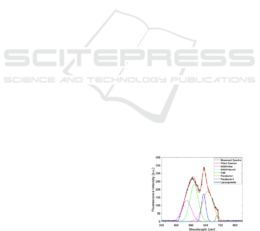
Figure 1: Spectrum fitted by a sum of six Gaussians.

PHOTOPTICS 2022 - 10th International Conference on Photonics, Optics and Laser Technology

scanned point by point with a 0.2 mm step along

several parallel lines spaced by 2 mm. The obtained

spectrum at each point is fitted by a sum of six

Gaussians functions, one for each fluorophore. The

integral under the curve and the maximum are

recorded for each Gaussian. Figure 1 illustrates an

acquired spectrum and the six Gaussian fitted curves.

The samples cohort consisted of 21 specimens

relative to four different pathologies: Diffuse Glioma

(DIF), Glioblastoma (GBM), Meningioma (MEN)

and metastasis (MET) and also one control group

(CTR) obtained from epileptic surgeries. Table 1

summarizes the samples cohort used for visible

spectral measurements.

The database in the visible domain totalizes 1701

records. These spectra are those for which data at both

375 and 405 nm are available exactly at the same

position on the same sample.

Table 1: Distribution of the data in the visible domain.

Number of tissue

specimens

Number of

spectrum

CTR

685

DIF

274

GBM

260

MEN

310

MET

172

Total

1701

2.2.2 DUV Range

The DUV measurements setup uses 275 nm as

excitation wavelength. Using this wavelength, we

were able to excite the following fluorophores:

Tyrosine (TYR), Tryptophan (TRY) collagen

crosslinks (COL) and NADH.

In each 10µm slice of each sample, a rectangular area

was chosen. This area was pixelated and spectral

acquisition were performed on each pixel.

Similar to the visible measurements, each spectrum

acquired in the DUV range was fitted by a sum of 4

Gaussians functions, one for each fluorophore, and

the integral under the curve and the maximum are

recorded for each Gaussian.

The samples cohort used in DUV measurements

includes five pathologies and one control group. The

pathologies represented in that group are: High grade

glioma (HGG), Low grade glioma (LGG),

Meningioma grade 2 (GII), Meningioma grade 1 (GI)

and Metastasis (MET) for a total of 38 patients. In

most cases, two slices were collected from each

samples, leading to a total of 67 tissue slices. The

complete DUV database include 129711 records.

Table 2 summarizes the samples cohort used for DUV

spectral measurements.

Table 2: Distribution of the data in the DUV domain.

Number of

patients

Number of

tissue

specimens

Number of

spectrum

CTR

21997

LGG

32051

HGG

21807

19872

GII

12784

MET

21200

Total

129711

2.3 Classification Method

The software was developed in Python. The Scikit-

learn library was used for pre-processing, feature

analysis and ML algorithm.

In a first step, the features were analysed by a pair-

to-plot method in order to roughly evaluate their

discriminating power and to highlight the obvious

correlation between them.

A multivariate analysis was then performed using

a non-parametric supervised ML approach commonly

used for classification problems and based on

Decision Trees (DT). DT are an important type of

algorithm for predictive modelling ML covering both

classification and regression topics. The goal of a DT

is to create a model that predicts the value of a target

variable by learning simple decision rules inferred

from the data features (Gordon, 1984). As the name

suggests, it uses a tree-like model of decisions and

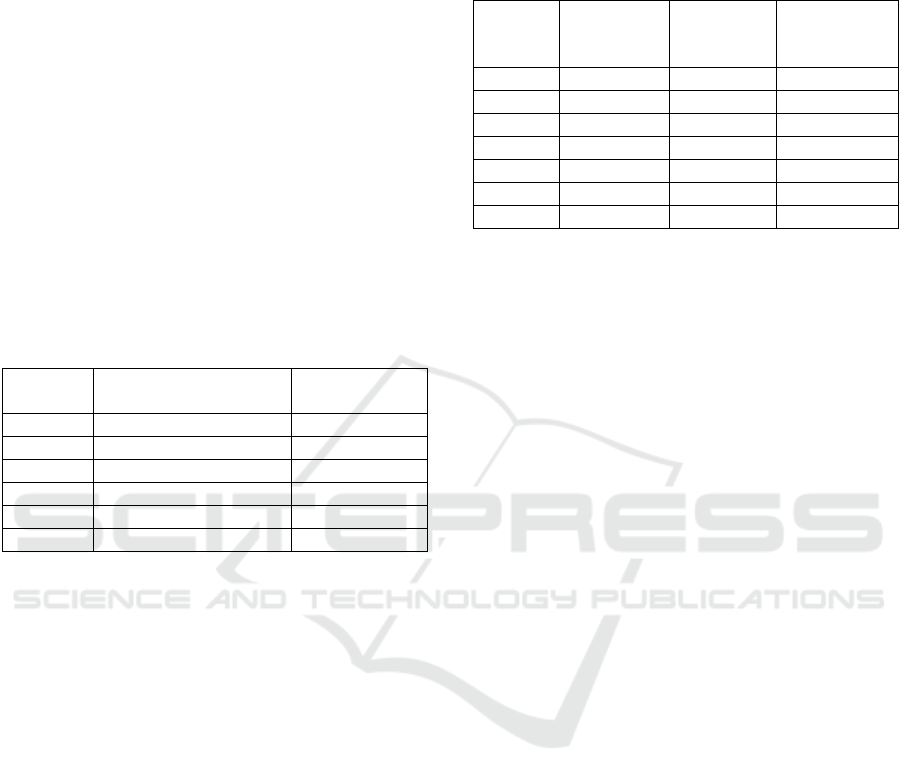
can be used to visually and explicitly represent them.

The structure of the DT is illustrated in figure 2. It is

drawn upside down with its root at the top. The input

subset is successively split into two branches (edges)

according to the condition present in each internal

node. The condition is a threshold on one of the

feature describing the samples. The end of the branch

that does not split anymore is the final decision (leaf)

for that branch. Tuning the model consists in getting

the most homogeneous branches as possible, in other

words branches having groups from similar classes.

The performance of the model is then evaluated on

unknown samples.

The classical DT algorithms have been around for

decades and modern variations like Random Forests

(RF) or Gradient Boosted Decision Trees (DT) are

currently among the most powerful techniques

available.

Classiﬁcation of Brain Tumour Tissues in Human Patients using Machine Learning

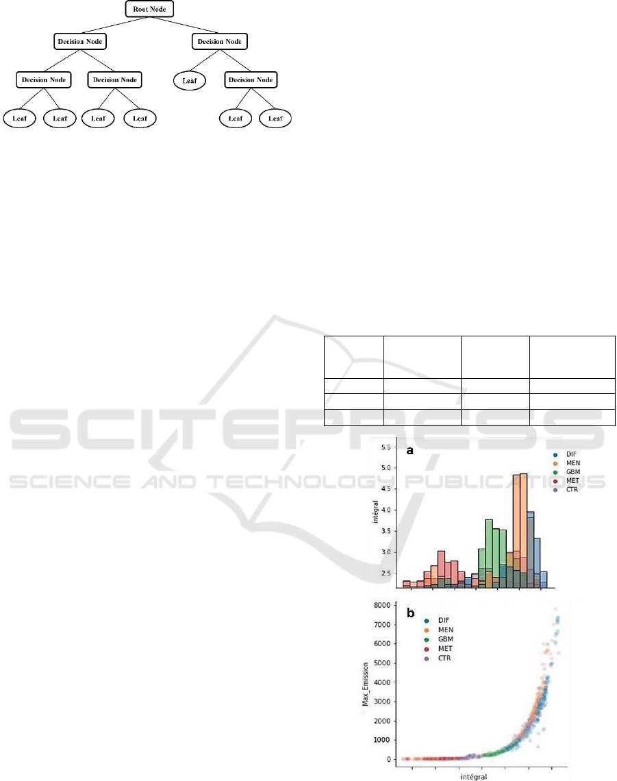
Figure 2: Decision Tree structure.

In RF algorithm, several DT are built in order to

decrease the variance thus yielding an overall better

model. The DT are built independently from a

random subset of the input samples and/or from a

random subset of the feature. The final classification

is obtained by averaging the probabilistic prediction

of all the DT (Breiman, 2001).

The GBDT algorithm is an iterative method

(Wolpert, 1992). The DT are built successively by

minimizing a differentiable loss function and a weight

is assigned to each DT for the final classification.

In Random Forest (RF) algorithm, several DT are

built in order to decrease the variance thus yielding an

overall better model. The DT are built independently

from a random subset of the input samples and/or

from a random subset of the feature. The final

classification is obtained by averaging the

probabilistic prediction of all the DT (Breiman,

2001). The Gradient Boosted Decision Trees (GBDT)

algorithm is an iterative method (Wolpert, 1992). The

DT are built successively by minimizing a

differentiable loss function and a weight is assigned

to each DT for the final classification.

3 RESULTS

3.1 Visible Range

Figure 3 shows a typical histogram and a pair-to-pair

plot (log scale) resulting from the preliminary

analysis. Figure 3.a suggests that the illustrated

feature (P2 here) can help discriminate the

pathologies. Figure 3.b clearly highlights that the

integral and the maximum of intensity are highly

correlated. That correlation was observed for each

fluorophore and each wavelength. We therefore only

kept the integral for the analysis.

The features that were taken into account in the

visible domain are the integral under the curve value

for each fluorophore at both 375 and 405 nm.

Previous studies proved that some ratio could also be

a powerful discriminatory feature (Poulon, 2018)

(Poulon, 2018) (Mehidine, 2021). We therefore

included four more parameters, namely the ratio

between integral of NADH-F and NADH-B and the

ratio between integral of P1 and P2 for both

wavelength, leading to a total number of 16 features

for each sample. The model was trained with 1360

samples (80% of the database) and evaluated on the

remaining 341samples (20%). DT achieves a 90%

score, RF 92% and GBDT 95% (Table 3).

We studied the importance of each feature for the

classification. The feature the most useful to build the

GBDT model is the ratio P1/P2 at 375nm. The next

one is integral of NADH-F at 375 nm. Though these

two features are the most useful, training the model

with only one of them or both of them leads to very

poor results (Table 3).

Table 3: Classification on the test database in the visible

domain for 1, 2 and 16 features using Decision Tree,

Random Forest and Gradient Boosting Decision Tree.

P1/P2

NADF_F

& P1/P2

16 features

47%

69%

90%

50%

73%

92%

GBDT

50%

71%

95%

Figure 3: P2 at 375 nm ; histogram of integral under the

curve (a) ; pair-to-pair plot for maximum if intensity versus

integral in a log-scale (b).

PHOTOPTICS 2022 - 10th International Conference on Photonics, Optics and Laser Technology

3.2 DUV Range

In the DUV, 8 features were included for each sample

into the model: the integral under the curve of each

of the 4 fluorophores and 4 ratio: TYR/NADH,

COL/NADH, TRY/COL, TYR/TRY. The model was

trained with 90797 samples (80% of the database) and

evaluated on the remaining 38914 samples (20%).

The 3 models achieve very similar score: 87% for

DT, 89% for RF and 88% for GBDT (Table 4).

We also studied the importance of each feature for

the classification. The features the more useful to

build the models are integral of collagene (COL) and

of tryptophane (TRY). Here also, training the model

with only those parameters leads to poor results.

Table 4: Classification on the test database in the DUV for

2 and 16 features using Decision Tree, Random Forest and

Gradient Boosting Decision Tree.

COL & TRY

16 features

49%

87%

42%

89%

GBDT

51%

88%

4 DISCUSSION AND

CONCLUSION

For the first time, we used ML methods on

spectroscopic data from brain tissue samples in order

to discriminate tumoral from non tumoral tissues

using quantitative optical parameters. This

preliminary study suggests that combining several

features into a ML model significantly improve the

classification.

We could not combine DUV and visible data in

the same model because we did not have the exact

position of the spectral records and we could not

establish the correspondence between two samples.

Such combination will be upgraded in the next

database. As the most discriminant features in DUV

and visible don’t come from the same fluorophores,

an improved result can be expected because it can be

assumed that useful information is complementary.

Indeed, though the input number of samples given

to the ML model is very high, they come from a

limited number of histological specimens and it is

necessary to confirm these results on more

specimens.

In this study, we only take into account spectral

data. Work is in progress to take advantage of other

available information such as fluorescence lifetime

and fluorescence and SHG optical images.

ACKNOWLEDGEMENTS

This work is financially supported by ITMO Cancer

AVIESAN (Alliance Nationale pour les Sciences de la Vie

et de la Santé, National Alliance for Life Sciences &

Health) within the framework of the Cancer Plan for

MEVO & IMOP projects, by CNRS with “Dfi

instrumental” grant, by ligue nationale contre le cancer

(LNCC) and the Institut National de Physique Nuclaire et

de Physique des Particules (IN2P3).

We would like to thank Synchrotron SOLEIL for the

accorded beam-time and for all staff members of DISCO

beamline for their help as well their contribution in the

scientific discussion. We would like also to thank the

Delegation for Clinical Research and Innovation (DRCI)

and the Biological Resources Center (CRB) of Sainte-Anne

hospital center for providing the samples.

We would to thank also the neurosurgeons at Sainte-

Anne hospital (M Zanello, E Dezamis, C Benevello, G Zah-

Bi, A Roux) for providing the surgical specimens.

REFERENCES

C. Buckner, et al., (2007) ‘Central Nervous System

Tumors’, Mayo Clin. Proc., vol. 82, no. 10, pp. 1271–

1286.

D. N. Louis et al., (2016), ‘The 2016 World Health

Organization Classification of Tumors of the Central

Nervous System: a summary’, Acta Neuropathol.

(Berl.), vol. 131, no. 6, pp. 803–820.

T. Wilson, M. Karajannis, and D. Harter, (2014),

‘Glioblastoma multiforme: State of the art and future

therapeutics’, Surg. Neurol. Int., vol. 5, no. 1, p. 64.

P. L. Kubben, et al., (2011), ‘Intraoperative MRI-guided

resection of glioblastoma multiforme: a systematic

review’, Lancet Oncol., vol. 12, no. 11, pp. 1062–1070,

G. Unsgaard et al., (2006), ‘Intra-operative 3D ultrasound

in neurosurgery’, Acta Neurochir. (Wien), vol. 148, no.

3, pp. 235–253

A. Ibrahim, et al., ‘Characterization of fiber ultrashort pulse

delivery for nonlinear endomicroscopy’, (2016), Opt.

Express, vol. 24, no. 12, p. 12515.

M. Sibai et al., (2018), ‘The Impact of Compressed

Femtosecond Laser Pulse Durations on Neuronal

Tissue Used for Two-Photon Excitation Through an

Endoscope’, Sci. Rep., vol. 8, no. 1, p. 11124.

F. Poulon et al., (2018), ‘Multimodal Analysis of Central

Nervous System Tumor Tissue Endogenous

Fluorescence With Multiscale Excitation’, Front.

Phys., vol. 6.

F. Poulon et al., (2018), ‘Real-time Brain Tumor imaging

with endogenous fluorophores: a diagnosis proof-of-

concept study on fresh human samples’, Sci. Rep., vol.

8, no. 1, p. 14888.

H. Mehidine et al., (2019), ‘Optical Signatures Derived

From Deep UV to NIR Excitation Discriminates

Healthy Samples From Low and High Grades Glioma’,

Sci. Rep., vol. 9, no. 1, p. 8786.

Classiﬁcation of Brain Tumour Tissues in Human Patients using Machine Learning

H. Mehidine et al., (2021), ‘Molecular changes tracking

through multiscale fluorescence microscopy

differentiate Meningioma grades and non-tumoral brain

tissues’, Sci. Rep., vol. 11, no. 1, p. 3816.

F. Poulon et al., (2017), ‘Optical properties, spectral, and

lifetime measurements of central nervous system

tumors in humans’, Sci. Rep., vol. 7, no. 1.

M. Zanello et al., (2017), ‘Multimodal optical analysis of

meningioma and comparison with histopathology’, J.

Biophotonics, vol. 10, no. 2, pp. 253–263.

H. Mehidine et al., (2018), ‘Multimodal imaging to explore

endogenous fluorescence of fresh and fixed human

healthy and tumor brain tissues’, J. Biophotonics, p.

e201800178.

A. D. Gordon, et al., (1984), ‘Classification and Regression

Trees.’ Biometrics, vol. 40, no. 3, p. 874.

L. Breiman, (2001), Mach. Learn., vol. 45, no. 1, pp. 5–32.

D. H. Wolpert, (1992), ‘Stacked generalization’, Neural

Netw., vol. 5, no. 2, pp. 241–259.

PHOTOPTICS 2022 - 10th International Conference on Photonics, Optics and Laser Technology