Variational Temporal Optical Flow for Multi-exposure Video

Onofre Martorell

and Antoni Buades

1 b

Institute of Applied Computing and Community Code (IAC3) and with the Dept.of Mathematics and Computer Science,

Universitat de les Illes Balears, Cra. de Valldemossa km. 7.5, E-07122 Palma, Spain

Keywords:

Optical Flow, Motion Estimation, Variational Methods, Multi-exposure Videos.

Abstract:

High Dynamic Range (HDR) reconstruction for multi-exposure video sequences is a very challenging task.

One of its main steps is registration of input frames. We propose a novel variational model for optical ﬂow

estimation for multi-exposure video sequences. We introduce data terms for consecutive and non consecutive

frames, the latter term comparing frames with the same exposure. We also compute forward and backward ﬂow

terms for the current frame, naturally introducing temporal regularization. We present a particular formulation

with sequences with two exposures, that can be extended to larger number of exposures. We compare the

proposed method with state of the art variational models.

1 INTRODUCTION

Multi-exposure fusion (MEF) and High Dynamic

Range (HDR) imaging are two techniques to combine

several images of the same scene taken with differ-

ent exposure times into a single image. Conventional

cameras are not able to capture in one shot the whole

large range of natural light present in the scene. Al-

though both families of methods seek the same goal,

the main procedure used is different. On one hand,

in HDR, the irradiance values of each image need to

be obtained. To do that, the camera response function

(CRF) has to be estimated, generally using the method

proposed by Devebec and Malik (Debevec and Ma-

lik, 2008). After the fusion, the result obtained by a

HDR method has to be converted into a standard 8

bit image, for visualization in common displays. This

process is known as tone-mapping (Reinhard et al.,

2005). On the contrary, MEF avoids the CRF esti-

mation and the tone-mapping by directly fusing the

images in the standard 8bit domain.

There exists a wide literature on MEF and HDR.

The most well-known method in MEF is the one pro-

posed by Mertens et al. (Mertens et al., 2009) and

in HDR, a widely used method is the one proposed

by Devebec and Malik (Debevec and Malik, 2008).

In order to apply both methods, the image sequence

needs to be static, that is, the objects in the scene do

not move and the camera is ﬁxed. This is not the case

https://orcid.org/0000-0002-9071-778X

https://orcid.org/0000-0001-9832-3358

for many sequences, and the application of such meth-

ods introduce ghosting effects. To avoid these arte-

facts, methods might be adapted to non-static image

sequences (Martorell et al., 2019), (Ma et al., 2017),

(Hu et al., 2013), (Khan et al., 2006).

A natural extension of MEF and HDR imaging

algorithms are MEF and HDR video, respectively.

There is a lack of specialized hardware to acquire

pleasant videos with large range of colors directly or it

is too expensive to be used in daily-used devices such

as mobile phones because they require complex sen-

sors or optical systems (Tocci et al., 2011)(Zhao et al.,

2015). The best way to overcome this problem is by

capturing videos where each frame is taken with alter-

nating exposure times (generally 2 or 3) and produce

a video with a high range of colors by processing the

frames ofﬂine using MEF or HDR techniques. Fig-

ure 1 shows some examples of muti-exposure video

sequences.

The transition from MEF or HDR imaging to the

corresponding video method is not straightforward.

First, only two or three exposures are available, mean-

ing that for some regions we will only dispose of un-

der or over exposed images. This is not the case for

still image combination where ﬁve or more exposures

might be available. Second, when a single image

needs to be synthesized, the image with the best expo-

sure of the initial set can be chosen as reference and

the rest be registered according to this reference one.

However, in HDR and MEF video, methods need to

be applied taking as reference each one of the frames,

666

Martorell, O. and Buades, A.

Variational Temporal Optical Flow for Multi-exposure Video.

DOI: 10.5220/0010908300003124

In Proceedings of the 17th International Joint Conference on Computer Vision, Imaging and Computer Graphics Theory and Applications (VISIGRAPP 2022) - Volume 4: VISAPP, pages

666-673

ISBN: 978-989-758-555-5; ISSN: 2184-4321

which are generally darker or brighter than a middle-

exposed image.

Registration is an important step in video fusion

and the overall result depends critically on it. Most

HDR video methods try to estimate the optical ﬂow

between the central frame and the neighbouring ones,

which were taken with a different exposure time. In

two exposure video sequences, this means the ﬂow

with the previous and posterior frames is computed.

Methods additionally compute the ﬂow between the

previous and posterior frames which have the same

exposure. Then methods select among computed ﬂow

locally depending if the regions is or not saturated.

We propose a variational method for optical ﬂow

with two alternating exposures. We combine in a

single functional the forward and backward ﬂow and

take advantage that the previous and posterior frames

have the same exposure. All computed ﬂows are de-

ﬁned taking the central image grid as reference, al-

lowing to naturally include temporal regularization.

This paper is organized as follows. In Section 2

we present the existing literature on registration for

multi-exposure video sequences and variational op-

tical ﬂow with temporal smoothness constraints. In

Section 3 we propose a new optical ﬂow variational

model for triplets of images in a video. In Section 4

we compare the obtained results with existing optical

ﬂow methods. Finally, in Section 5 we draw some

conclusions and future work.

2 RELATED WORK

2.1 HDR Video

It is not surprising that no methods are proposed for

dealing with multi-exposure sequences directly in the

input 8 bit domain. MEF methods perform worse than

HDR when few exposures are available, which is the

case of video. However, there are many works which

deal with HDR for video sequences. We will make a

review of those methods, focusing on the techniques

used to register the input images. All those meth-

ods use an estimation of the CRF to transform the

input images from an LDR domain to an HDR do-

main. These radiance frames are then normalized by

dividing by its exposition time. In this way, different

frames have the same irradiance value at correspond-

ing pixels.

The common step for reducing ghosting artifacts

is registering the frames prior to their combination.

The classical method for HDR video registration is

the use of optical ﬂow, e.g Lukas-Kanade, used by

Kang et al. (Kang et al., 2003), block matching, used

by Mangiat et al. (Mangiat and Gibson, 2010) or the

method proposed by Liu (Liu et al., 2009), used by

Kalantari et al. (Kalantari et al., 2013). The more re-

cent Li et al. (Li et al., 2016) ﬁrst separate foreground

and background before registering the frames.

Musil et al. (Musil et al., 2020) present a fast

ghost-free HDR acquisition algorithm for static cam-

eras. For each frame, they compute a certainty map

based on the difference of pixel values with its neigh-

boring frames in the radiance domain. This permits

the removal of moving objects and the fusion to ob-

tain the ﬁnal HDR image.

Van Vo and Lee (Van Vo and Lee, 2020) is the

only method that takes into account the temporal in-

formation: they divide the motion estimation step into

two phases: on one hand, they perform optical ﬂow

estimation of well-exposed areas in the descriptor do-

main. On the other hand, they perform a superpixel-

based motion estimation on poorly exposed areas by

computing the optical ﬂow ﬁeld from the backward

frame to the forward frame. The optical ﬂow from

central to forward and backward frames is half of the

computed ﬂow.

There exist learning-based methods for HDR

video synthesis (Kalantari and Ramamoorthi, 2019)

(Chen et al., 2021). In both cases, they compute the

optical ﬂow of the input frames by training a CNN

coarse-to-ﬁne architecure based on the ones by Ran-

jan and Black (Ranjan and Black, 2017) and Wang et

al. (Wang et al., 2017). Training is performed into

an end-to-end way, meaning that only the error of the

ﬁnal HDR sequence is used for deﬁning the loss.

2.2 Variational Optical Flow with

Temporal Regularization

The ﬁrst variational formulation of the optical ﬂow

problem was presented by Horn and Schunk (Horn

and Schunck, 1981). They proposed to ﬁnd the op-

tical ﬂow ﬁeld w = (u, v) between a pair of images,

and I

, by minimizing an energy functional formed

by two different terms: the data and the smoothness

terms. The ﬁrst one imposes the brightness constancy

constraint, that is, the gray values of corresponding

pixels are the same; and the second one penalizes the

high variations of the optical ﬂow ﬁeld. This second

term was written as

Ω

(||∇u(x)||

+ ||∇v(x)||

)dx, (1)

with x = (x, y) being a two-dimensional point.

Weickert and Schn

orr (Weickert and Schn

orr,

2001) proposed the ﬁrst method introducing a tem-

poral derivative in the energy functional. Instead of

computing the optical ﬂow between a pair of frames,

Variational Temporal Optical Flow for Multi-exposure Video

667

bridge2hallway2

hands

ninja

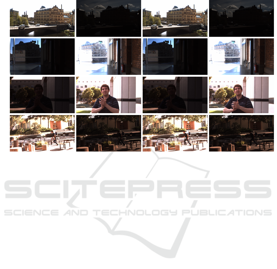
Figure 1: Frames of multi-exposure video sequences with 2 exposure times used for comparison. Sequences obtained from

Kalantari et al. (Kalantari et al., 2013) and Li et al. (Li et al., 2016) datasets.

they considered a video sequence {I

| t = 0, . . . , N}.

They used the data term proposed in (Horn and

Schunck, 1981) but used a 3D gradient operator for

the smoothness term:

Ω×[0,N]

Ψ(||∇

u(x)||+ ||∇

v(x)||)dx, (2)

with x = (x, y, t) being a three-dimensional point,

where the third coordinate corresponds to the time.

Brox et al. (Brox et al., 2004) adopted the same reg-

ularity term as Weickert and Schn

orr but introduced a

new data term based on the correspondence of gradi-

ents. In both cases, this regularization operator may

fail in presence of large and complex motions.

Salgado et al. (Salgado and S

anchez, 2007) pro-

pose to separate the temporal regularization constraint

from the spatial one in (2). They used the same spatial

regularization term as in (1) and proposed the tempo-

ral term

Ω

N−1

∑

t=0

Ψ(||w

(x) −w

t+1

(x + w

(x))||

)dx+

Ω

∑

t=1

Ψ(||w

(x) −w

t−1

(x + w

∗

t−1

(x))||

)dx,

where w

∗

i−1

(x) is the backward ﬂow. This new tem-

poral term is nonlinear but permits to better deal with

large displacements. Moreover, for small displace-

ments, this term can be seen as the discretization of

the temporal derivative presented previously. Years

later, Sanchez et al. (S

anchez et al., 2013) improved

the method by introducing a second order temporal

smoothness constraint at the PDE level:

N−1

∑

t=1

(||w

t−1

(x + w

∗

t−1

(x)) −w

t+1

(x + w

(x))||

)·

t−1

(x + w

∗

t−1

x)) −2w

+ w

t+1

(x + w

x))).

(3)

Volz et al. (Volz et al., 2011) proposed a

novel parametrization of optical ﬂow ﬁelds to encour-

age temporal regularization along motion trajectories.

With this new parametrization, the nonlinearity form

Sanchez et al. disappears and the minimization be-

comes simpler. As Sanchez et al., they also used

a second order regularization, in this case added di-

rectly in the energy functional:

Ω

N−1

∑

t=0

Ψ(||w

t+1

(x) −w

(x)||

)dx+

Ω

N−1

∑

t=1

Ψ(||w

t+1

(x) −2w

(x) + w

t−1

(x)||

)dx.

(4)

3 OPTICAL FLOW WITH

TEMPORAL CONSTRAINTS

Let {I

|t = 0, . . . , N} be a sequence of images, where

images are taken with 2 different alternating exposure

VISAPP 2022 - 17th International Conference on Computer Vision Theory and Applications

668

times. Figure 1 shows some examples of frames of

the videos used in the experimentation section. At

each frame position we dispose of a single exposure.

Hence, we need to compute optical ﬂow between con-

secutive frames of different exposure.

Let I

be the reference frame and I

t+1

and I

t−1

the previous and posterior frames, respectively. We

present the method for this triplet of images, and it is

repeated for each t ∈ {1, . . . , N −1}.

It must be noted that most variational optical ﬂow

models rely on the brightness constancy assumption,

which states that two corresponding pixels have the

same color. However, this assumption is not satis-

ﬁed with multi-exposure images. To overcome this

issue, we apply photometric calibration to the pairs

, I

t+1

) and (I

, I

t−1

) separately by using the method

proposed by Martorell et al. (Martorell et al., 2019).

As most algorithms, we choose to modify the color of

the darker images of the sequence, to look alike the

neighbouring brighter ones. Brighter images might

have large saturated areas while this is not the case of

darker ones.

The used method for photometric calibration re-

quires that the input images are roughly registered.

Hence, we ﬁrst globally register the neighbour frames

with respect to the reference one. We use a global

afﬁne transformation. This is estimated using SIFT

matches (Lowe, 1999) and RANSAC strategy (Fis-

chler and Bolles, 1981). After this initial registration

we apply the photometric calibration from Martorell

et al. (Martorell et al., 2019).

Once the images are photometrically calibrated

and globally registered, we can estimate the optical

ﬂow between neighbouring frames using a variational

model.

3.1 Proposed Variational Model

Let I

t−1

, I

and I

t+1

be 3 consecutive frames from a

multi-exposure video sequence and let w

(x) be the

optical ﬂow ﬁeld from I

(x) to I

t+1

(x) and w

(x) the

optical ﬂow ﬁeld from I

(x) to I

t−1

(x). We want to

jointly estimate the optical ﬂow ﬁelds from the cen-

tral frame to the other two by taking into account the

video nature of the input data. Apart from the well-

known data and spatial smoothness terms, we want to

impose two new aspects in the minimization. On one

hand, we want that the motion trajectories are smooth

along the video sequence. On the other hand, we want

to match pixels from I

t−1

to I

t+1

Most methods presented in Section 2.2

parametrize w

(x) as the optical ﬂow from I

t−1

(x)

to I

(x), but this forces them to minimize the energy

functional twice, in order to warp both neighbour

frames. In our case, we follow the parametriza-

tion from Volz et al. (Volz et al., 2011), which

parametrizes both optical ﬂow ﬁelds with regard to

the central frame and allows to warp both neighbour

frames by minimizing just one energy functional.

Most methods for HDR video compute separately

the registration ﬁelds w

(x) and w

(x). However,

these estimations are prone to fail at saturated areas.

To solve this, Van Vo and Lee (Van Vo and Lee, 2020)

also compute the optical ﬂow from I

t−1

(x) to I

t+1

(x)

and combine it heuristically with w

(x) and w

(x).

In contrast, the proposed method introduces the com-

parison of non-consecutive frames in the energy func-

tional to address this problem.

With all that, we propose to minimize the fol-

lowing energy functional to estimate the optical ﬂow

ﬁelds:

E(w

, w

) = α



S (w

) + S (w

)



+ δT (w

, w



) + γ

) + λJ (w

, w

)



(5)

where variables β, γ

, γ

, λ, α and δ are the

weights that measure the trade-off of each term and

) =

Ω





t+1,t

(x + w

) −

t,t+1

(x)





(6)

) =

Ω





t−1,t

(x −w

) −

t,t−1

(x)





(7)

J (w

, w

) =

Ω



t+1

(x + w

) −I

t−1

(x −w

))



(8)

S (w) =

Ω



||∇w



+ Ψ



||∇w



dx (9)

T (w

, w

) =

Ω



||w

−w



dx (10)

where

k j

and

are pairs of images I

and I

photometrically calibrated according to the criteria

presented at the beginning of the section. Finally,

Ψ(s

) =

√

+ ε

with ε = 0.00001 is a robust convex

function.

The proposed energy functional contains several

terms which serve for different purposes, let’s analyse

in detail all the terms of the energy functional:

(i) D

): data term to match pixels from

t,t+1

t+1,t

through optical ﬂow ﬁeld w

(ii) D

): data term to match pixels from

t,t−1

t−1,t

through optical ﬂow ﬁeld w

. Since w

Variational Temporal Optical Flow for Multi-exposure Video

669

is computed with regard to the central frame, we

need to substract the optical ﬂow to the coordi-

nates to get the right registration.

(iii) J (w

, w

): data term to match pixels from I

t+1

and I

t−1

through optical ﬂow ﬁelds w

and w

Since both optical ﬂow ﬁelds have the same ref-

erence, we can use this term easily, without in-

troducing nonlinearities, which could make the

minimization more difﬁcult.

(iv) S (w): spatial smoothness term for optical ﬂow.

(v) T (w

, w

): ﬁrst order temporal smoothness

term to regularize motion trajectories. Since

both optical ﬂow ﬁelds have the same reference,

we just need to substract them, not as in Sanchez

et al. (S

anchez et al., 2013), where they needed

to compose optical ﬂow ﬁelds to write this term.

3.2 Minimization

The minimization of the energy functional (5) at each

frame I

is done by ﬁnding the corresponding Euler-

Lagrange equation and solving the obtained linear

system of equations with a successive over-relaxation

(SOR) scheme. The minimization is embedded in

a pyramidal structure to better deal with large dis-

placements: given a number of scales N

scales

, and

a downsampling factor ν, the input images at scale

s = 0, . . . , N

scales

−1 are the input images at scale s−1

convolved with a Gaussian kernel and downsampled

by a factor ν. We start estimating the optical ﬂow

at scale s = N

scales

−1, then we upsample the output

ﬂow and we repeat the minimization at scale s −1 by

using as initialization the upsampled optical ﬂow.

4 RESULTS

In this section we compare the proposed fusion al-

gorithm with other variational optical ﬂow methods.

We compare our method against Brox et al. (Brox

et al., 2004) with and without temporal smoothness

constraints. In both cases, we use the implementa-

tion available at ipol.im (S

anchez P

erez et al., 2013).

We modiﬁed the code of the method with temporal

constraints to be able to deal with pairs of photome-

trically calibrated images, as in the proposed model.

For simplicity, we name the methods brox spatial and

brox temporal, respectively. In both methods we need

to compute two ﬂows: in brox spatial we need to

compute separately the ﬂow from I

to I

t+1

and from I

to I

t−1

. On the other hand, brox temporal model gives

always the optical ﬂow from one frame to the next

Table 1: Mean error of 4 frames from each sequence. In

bold, the method with lowest error for each sequence.

Brox et al.

temporal

Ours

hands 10.67 13.68 11.99

ninja 23.30 32.10 20.88

bridge 15.25 18.95 13.93

hallway 10.71 12.59 10.71

parkinglot 24.30 31.67 22.94

Average 14.04 18.17 13.41

one. Hence, we need to apply the model to the se-

quence {I

t−1

, I

t+1

} and to {I

t+1

, I

t−1

} to get w

and w

We evaluate our algorithm by using several multi-

exposure video sequences available online: Kalantari

et al. (Kalantari et al., 2013) have available online

a dataset of 7 sequences, 4 of them with 2 exposures.

We use sequences hands and ninja from this dataset.

Moreover, Li et al. (Li et al., 2016) have available

online

a dataset with 4 video sequences with 2 ex-

posure times. From this dataset, we use sequences

bridge, hallway and parkinglot.

Our results were computed using the same param-

eters for all tests. We set weights β, α and δ to 1,

13 and 0.5, respectively. The values of γ

, γ

and λ

have been set taking into account the kind of input

data used: in multi-exposure videos sequences with

2 exposure times, frames I

t−1

and I

t+1

have the same

exposure times, hence, their comparison will be more

reliable compared to the ones of consecutive frames,

which have different exposure times. Because of that,

we have decided to give more weight to the term

J (w

, w

) by setting λ = 1 and γ

= γ

= 0.5.

We ﬁrst evaluate our algorithm quantitatively in

4 images of different sequences. We compute all

needed optical ﬂow ﬁelds at each frame, we then com-

pute the registration error for each frame and we ﬁ-

nally do the mean to get a measure of the error on

each sequence. For each frame I

, we compute the

error as

∑

x∈

Ω



t+1,t

(x + w

) −

t,t+1

(x)



∑

x∈

Ω



t−1,t

(x −w

) −

t,t−1

(x)



(11)

where

Ω is the discrete domain of the image.

Table 1 shows the results on 5 multi-exposure se-

quences, where the method with lowest error is high-

lighted in bold. As we can see, our methods obtains

the lowest error in 4 sequences. In hands sequence we

https://web.ece.ucsb.edu/∼psen/PaperPages/HDRVideo

http://signal.ee.psu.edu/research/MAPHDR.html

VISAPP 2022 - 17th International Conference on Computer Vision Theory and Applications

670

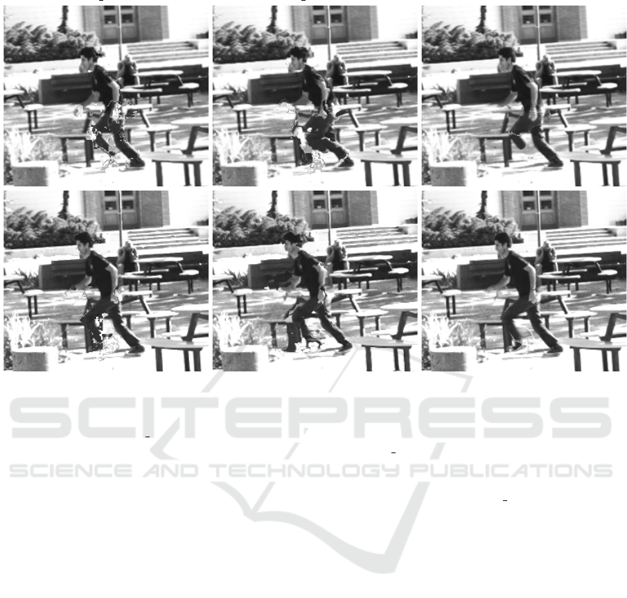
brox spatial brox temporal Ours

Figure 2: Warped images for two consecutive frames of ninja sequence.

get the second best error, and in hallway sequence we

get the same error as brox spatial.

We also evaluate our results qualitatively. Figure

2 shows a detail of I

t−1

(x − w

) for two consecu-

tive frames of ninja sequence. As it can be seen, our

method performs better than the compared methods.

We also evaluate our optical ﬂow method by ﬁnd-

ing pixels with inaccurate displacement: we perform

a left-right consistency on the forward ﬂow as

LR(x) =max



||w

(x) + w

t+1

(x + w

)||, (12)

||w

(x) + w

t−1

(x + w

(x))||



(13)

(x) =



1 if LR(x) < 2

0 otherwise

. (14)

and the left-right consistency check on the backward

ﬂow M

is computed analogously. Since we have two

masks, we combine them to get a ﬁnal mask as

(x) = M

(x) ·M

(x). (15)

We apply the HDR algorithm from Khan et al.

(Khan et al., 2006) to the triplet of aligned images

to get a fusion with a large range of colors.

Figure 3 shows the result of fusing the three reg-

istered images using the HDR algorithm from Khan

et al. (Khan et al., 2006) as well as the left-right

consistency mask superimposed in two consecutive

frames of ninja sequence. As it can be seen, our

method has a better left-right consistency and align-

ment. Brox spatial has more errors at registration: the

stairs in the background at the second row are not per-

fectly aligned and the man has registration errors be-

tween the legs. Moreover, brox temporal has a small

misalignment on the right side of the second image,

making it look blurry. Finally, our method has less

errors due to left-right consistency.

5 CONCLUSIONS

We have presented a new variational model for opti-

cal ﬂow estimation in multi-exposure sequences. We

use temporal constraints to take into account the video

nature of input images. We have applied photometric

calibration to obtain pairs of images with the same

color, in order to satisfy brightness constancy on the

optical ﬂow model. Qualitative and quantitative per-

formance show that our method performs better than

other optical ﬂow variational models.

In future work, we plan to adapt the proposed

method for multi-exposure video sequences with 3

exposure times. In this case, forward and backward

frames do not have the same exposure time, hence we

need to use more frames in order to add more data

Variational Temporal Optical Flow for Multi-exposure Video

671

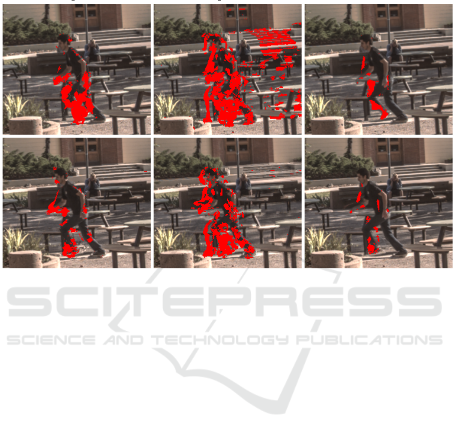
brox spatial brox temporal Ours

Figure 3: HDR fusion of registered images and left-right consistency mask superimposed in two consecutive frames of ninja

sequence.

terms like the one that matches pixels from forward

and backward frames.

Moreover, as seen in the results shown, our

method still has some registration errors, that should

be solved so as to get a good looking ﬁnal fused im-

age. To do that, we plan to apply some processing

techniques to remove them.

ACKNOWLEDGEMENTS

The authors acknowledge the Ministerio de Ciencia,

Innovaci

on y Universidades (MCIU), the Agencia Es-

tatal de Investigaci

on (AEI) and the European Re-

gional Development Funds (ERDF) for its support to

the project TIN2017-85572-P.

REFERENCES

Brox, T., Bruhn, A., Papenberg, N., and Weickert, J. (2004).

High accuracy optical ﬂow estimation based on a the-

ory for warping. In European conference on computer

vision, pages 25–36. Springer.

Chen, G., Chen, C., Guo, S., Liang, Z., Wong, K.-Y. K.,

and Zhang, L. (2021). Hdr video reconstruction: A

coarse-to-ﬁne network and a real-world benchmark

dataset. In Proceedings of the IEEE/CVF Interna-

tional Conference on Computer Vision (ICCV), pages

2502–2511.

Debevec, P. E. and Malik, J. (2008). Recovering high dy-

namic range radiance maps from photographs. In

ACM SIGGRAPH 2008 classes, page 31. ACM.

Fischler, M. A. and Bolles, R. C. (1981). Random sample

consensus: a paradigm for model ﬁtting with appli-

cations to image analysis and automated cartography.

Communications of the ACM, 24(6):381–395.

Horn, B. K. and Schunck, B. G. (1981). Determining optical

ﬂow. Artiﬁcial intelligence, 17(1-3):185–203.

Hu, J., Gallo, O., Pulli, K., and Sun, X. (2013). Hdr

deghosting: How to deal with saturation? In Pro-

ceedings of the IEEE Conference on Computer Vision

and Pattern Recognition, pages 1163–1170.

Kalantari, N. K. and Ramamoorthi, R. (2019). Deep hdr

video from sequences with alternating exposures. In

Computer Graphics Forum, volume 38, pages 193–

205. Wiley Online Library.

Kalantari, N. K., Shechtman, E., Barnes, C., Darabi, S.,

Goldman, D. B., and Sen, P. (2013). Patch-based high

dynamic range video. ACM Trans. Graph., 32(6):202–

Kang, S. B., Uyttendaele, M., Winder, S., and Szeliski, R.

(2003). High dynamic range video. In ACM Transac-

tions on Graphics (TOG), volume 22, pages 319–325.

ACM.

Khan, E. A., Akyuz, A. O., and Reinhard, E. (2006). Ghost

removal in high dynamic range images. In 2006 In-

VISAPP 2022 - 17th International Conference on Computer Vision Theory and Applications

672

ternational Conference on Image Processing, pages

2005–2008. IEEE.

Li, Y., Lee, C., and Monga, V. (2016). A maximum a pos-

teriori estimation framework for robust high dynamic

range video synthesis. IEEE Transactions on Image

Processing, 26(3):1143–1157.

Liu, C. et al. (2009). Beyond pixels: exploring new repre-

sentations and applications for motion analysis. PhD

thesis, Massachusetts Institute of Technology.

Lowe, D. G. (1999). Object recognition from local scale-

invariant features. In Proceedings of the seventh

IEEE international conference on computer vision,

volume 2, pages 1150–1157. Ieee.

Ma, K., Li, H., Yong, H., Wang, Z., Meng, D., and Zhang,

L. (2017). Robust multi-exposure image fusion: A

structural patch decomposition approach. IEEE Trans.

Image Processing, 26(5):2519–2532.

Mangiat, S. and Gibson, J. (2010). High dynamic range

video with ghost removal. In Applications of Digital

Image Processing XXXIII, volume 7798, page 779812.

International Society for Optics and Photonics.

Martorell, O., Sbert, C., and Buades, A. (2019). Ghosting-

free dct based multi-exposure image fusion. Signal

Processing: Image Communication, 78:409–425.

Mertens, T., Kautz, J., and Van Reeth, F. (2009). Expo-

sure Fusion: A Simple and Practical Alternative to

High Dynamic Range Photography. Computer Graph-

ics Forum.

Musil, M., Nosko, S., and Zemcik, P. (2020). De-ghosted

hdr video acquisition for embedded systems. Journal

of Real-Time Image Processing, pages 1–10.

Ranjan, A. and Black, M. J. (2017). Optical ﬂow estimation

using a spatial pyramid network. In Proceedings of

the IEEE conference on computer vision and pattern

recognition, pages 4161–4170.

Reinhard, E., Ward, G., Pattanaik, S., and Debevec, P.

(2005). High Dynamic Range Imaging: Acquisi-

tion, Display, and Image-Based Lighting (The Mor-

gan Kaufmann Series in Computer Graphics). Mor-

gan Kaufmann Publishers Inc., San Francisco, CA,

USA.

Salgado, A. and S

anchez, J. (2007). Temporal constraints in

large optical ﬂow estimation. In International Confer-

ence on Computer Aided Systems Theory, pages 709–

716. Springer.

anchez, J., Salgado de la Nuez, A. J., and Monz

on, N.

(2013). Optical ﬂow estimation with consistent spatio-

temporal coherence models.

anchez P

erez, J., Monz

on L

opez, N., and Salgado de la

Nuez, A. (2013). Robust Optical Flow Estimation.

Image Processing On Line, 3:252–270.

Tocci, M. D., Kiser, C., Tocci, N., and Sen, P. (2011). A

versatile hdr video production system. ACM Transac-

tions on Graphics (TOG), 30(4):1–10.

Van Vo, T. and Lee, C. (2020). High dynamic range

video synthesis using superpixel-based illuminance-

invariant motion estimation. IEEE Access, 8:24576–

24587.

Volz, S., Bruhn, A., Valgaerts, L., and Zimmer, H. (2011).

Modeling temporal coherence for optical ﬂow. In

2011 International Conference on Computer Vision,

pages 1116–1123. IEEE.

Wang, T.-C., Zhu, J.-Y., Kalantari, N. K., Efros, A. A., and

Ramamoorthi, R. (2017). Light ﬁeld video capture

using a learning-based hybrid imaging system. ACM

Transactions on Graphics (TOG), 36(4):1–13.

Weickert, J. and Schn

orr, C. (2001). Variational optic ﬂow

computation with a spatio-temporal smoothness con-

straint. Journal of mathematical imaging and vision,

14(3):245–255.

Zhao, H., Shi, B., Fernandez-Cull, C., Yeung, S.-K., and

Raskar, R. (2015). Unbounded high dynamic range

photography using a modulo camera. In 2015 IEEE

International Conference on Computational Photog-

raphy (ICCP), pages 1–10. IEEE.

Variational Temporal Optical Flow for Multi-exposure Video

673