A Smart Home Testbed for Evaluating XAI with Non-experts

Kevin McAreavey, Kim Bauters and Weiru Liu

Department of Engineering Mathematics, University of Bristol, U.K.

Keywords:

Explainable AI (XAI), Explainable Machine Learning, Explainable AI Planning (XAIP), Smart Homes.

Abstract:

Smart homes are powered by increasingly advanced AI, yet are controlled by, and affect, non-experts. These

non-expert home users are an under-represented stakeholder in the explainable AI (XAI) literature. In this

paper we facilitate future XAI research by introducing a family of smart home applications serving as a testbed

to evaluate XAI with non-experts. The testbed is a hybrid-AI system spanning several AI disciplines, including

machine learning and AI planning. Applications include a smart home battery and smart thermostatic radiator

valve (TRV). End-user functionality is representative of leading commercial products and relevant research

applications. The testbed is based on a ﬂexible software architecture and web-based user interface, supports a

range of AI tools in a modular fashion, and can be easily deployed using inexpensive consumer hardware.

1 INTRODUCTION

Research into explainable AI (XAI) has seen rapid

growth in recent years (Arrieta et al., 2020; An-

jomshoae et al., 2019; Adadi and Berrada, 2018) yet

signiﬁcant challenges still remain (Miller, 2019; Lip-

ton, 2018; Abdul et al., 2018), not least with regards

to evaluation (Hoffman et al., 2018).

Challenge 1: There is a need for explanations across

a wide range of AI subﬁelds, including but not lim-

ited to machine learning (Biran and Cotton, 2017), AI

planning (Chakraborti et al., 2020), multi-agent sys-

tems (Kraus et al., 2020), and robotics (Anjomshoae

et al., 2019). Mirroring broader trends in AI, machine

learning is certainly the dominant branch of current

XAI research (Chakraborti et al., 2020), but for many

domains this trend is not necessarily representative of

deployed AI systems. For example, the general public

is increasingly exposed to AI via smart home appli-

cations (Guo et al., 2019), but in this domain there is

evidence that the use of symbolic AI is still more com-

mon than machine learning (Mekuria et al., 2019).

Hybrid AI systems (i.e. those combining several AI

subsystems) are also common in this setting (Mekuria

et al., 2019).

Challenge 2: AI systems typically involve a wide

range of stakeholders—both expert and non-expert—

and the types of explanations appropriate to each class

of stakeholder may differ signiﬁcantly (Langer et al.,

2021). Recent machine learning research on XAI

has unfortunately tended to emphasise AI developers

at the expense of other stakeholders, especially non-

experts (Cheng et al., 2019). Arguably this reﬂects

a motivation centred on systems engineering, where

the outputs are intended to help machine learning ex-

perts better understand and debug their own systems,

rather than for e.g. non-experts to accept or trust the

adoption of those systems (Abdul et al., 2018). In the

smart home setting, studies have found that AI sys-

tems may frustrate and disempower non-experts due

to a lack of transparency (Yang and Newman, 2013).

Challenge 3: Evaluation of XAI research depends on

the existence of some core AI system that can pro-

vide functionality (its primary task) to stakeholders

regardless of any supplementary XAI features (Hoff-

man et al., 2018). This implies substantial overhead

for researchers around the development and/or de-

ployment of core AI systems that can sufﬁciently en-

gage target stakeholders and thus justify the need for

actual XAI features. While AI developers can be ex-

pected to engage with raw AI components, non-expert

stakeholders will typically engage with AI technol-

ogy indirectly via end-user features. This suggests

that evaluating XAI with non-expert stakeholders is

more time consuming than with AI developers, which

may partially explain the imbalance in current XAI

research (i.e. the low-hanging fruit argument). In any

case, it makes sense that a core AI system should be

representative of the kinds of AI system that a given

class of stakeholder will typically encounter.

In this paper we address the above challenges by

proposing a realistic smart home testbed to evaluate

McAreavey, K., Bauters, K. and Liu, W.

A Smart Home Testbed for Evaluating XAI with Non-experts.

DOI: 10.5220/0010908100003116

In Proceedings of the 14th International Conference on Agents and Artiﬁcial Intelligence (ICAART 2022) - Volume 3, pages 773-784

ISBN: 978-989-758-547-0; ISSN: 2184-433X

773

XAI with non-experts. Non-experts are chosen as an

important but under-represented class of stakeholder

within XAI research, while the smart home domain

is chosen as a leading source of AI faced by non-

experts. The testbed itself is comprised of two appli-

cations, namely a smart home battery offering elec-

tricity cost savings, and a smart thermostatic radiator

valve (TRV) for comfort and convenience. End-user

functionality is representative of leading commercial

smart home products, such as the Nest Learning Ther-

mostat, as well as relevant smart home applications in

the literature (e.g. Rogers et al., 2013; Shann et al.,

2017). Both applications have similar hybrid-AI de-

signs, comprised of low-level machine learning com-

ponents feeding into a high-level AI planning compo-

nent, while the underlying AI tools and algorithms are

modular. This design ensures that the testbed is appli-

cable to a wide range of AI and XAI methods. In

addition, we provide a software architecture and web-

based user interface that allows the testbed to be easily

deployed using inexpensive consumer hardware. This

alleviates many overheads encountered by researchers

when attempting to deploy AI systems in practice.

The remainder of the paper is organised as fol-

lows: in Section 2 we recall some relevant back-

ground from AI; in Section 3 we formalise our two

applications; in Section 4 we describe the overall

testbed; in Section 5 we discuss related work; and in

Section 6 we conclude, mentioning planned use of the

testbed in a scheduled research study on AI threats.

2 PRELIMINARIES

This section recalls some background on AI planning.

A (deterministic, cost-minimising) Markov decision

process or MDP is a tuple (S,A,T,C) where S is a set

of states, A is a set of actions, T : S × A → S is a tran-

sition function, and C : S × A → R is cost function.

Solutions to MDPs are optimal policies but are only

well-deﬁned for certain classes of MDP, with the typi-

cal examples being ﬁnite-horizon MDPs and (inﬁnite-

horizon) discounted-reward MDPs. In this paper we

are interested in the former. A ﬁnite-horizon MDP ex-

tends the standard MDP deﬁnition by including a (de-

cision) horizon t

max

∈ N with D = {1,. .. ,t

max

} the set

of timesteps. A (non-stationary) policy is a function

π : S × D → A where the cumulative cost of π in state

s ∈ S at timestep t ∈ N is deﬁned as:

V (s,t, π) =







C(s, a)

+V (s

,t + 1,π)

if 1 ≤ t ≤ t

max

0 otherwise

(1)

such that a = π(s,t) and s

= T (s,a). A policy π

∗

is an

optimal policy if it minimises V (s,t,π

∗

) for all s ∈ S

and all t ∈ D. A ﬁnite-horizon MDP can be further

extended to include some initial state s

∈ S, in which

case solutions may be simpliﬁed to only account for

states that are reachable from s

. A policy is partial

if π(s,t) = undeﬁned for some state s ∈ S and some

timestep t ∈ D. A partial policy is closed with re-

spect to state s

∈ S if π(s,t) 6= undeﬁned for any state

s ∈ S and any timestep t ∈ D such that (s,t) is reach-

able from (s

,1) while executing π. Since the above

transition function is deterministic, any partial policy

π that is closed with respect to initial state s

∈ S can

be represented by a sequence of actions of length t

max

An optimal partial policy that is closed with respect to

state s

∈ S is thus a sequence of actions of length t

max

that minimises cost when executed from s

. Comput-

ing such a policy is equivalent to a variant of classi-

cal AI planning where states are time-indexed states

S×D, the goal is S ×{t

max

}, and the language permits

both costs and continuous state variables.

3 APPLICATIONS

This section introduces our two testbed applications,

formalises the technical details of their underlying AI

components, and provides some experimental results.

3.1 Smart Home Battery

Energy markets in Europe and beyond establish prices

through an auction process divided into half-hour

blocks. Prices thus change every half-hour and it is

the energy supplier who hedges the risk of ﬂuctuating

prices on the inter-day market. With the emergence

of smart meters it has become possible for energy

providers, such as Octopus Energy in the UK or Engie

in Belgium, to introduce tariffs where the customer is

rewarded for consuming electricity when wholesale

prices are low by directly linking the customer tar-

iff to these half-hour blocks. The resulting tariffs are

known as dynamic or time-of-use tariffs and allow the

customer to reduce costs by scheduling ﬂexible elec-

tricity consumption (e.g. washing machine cycles) so

as to beneﬁt from price ﬂuctuations.

In the case of Octopus Energy, prices are allocated

each day and cover the subsequent 24 hours. Prices

are determined by wholesale prices, which in turn de-

pend on external factors (e.g. availability of renew-

ables). Additionally, customers are permitted to sup-

ply electricity to the grid (e.g. generated by domestic

solar panels) where they are charged for consumption

according to import prices and receive payment for

ICAART 2022 - 14th International Conference on Agents and Artiﬁcial Intelligence

774

supply according to export prices. Import prices have

an upper-bound of 35p/kWh and permit negative pric-

ing, meaning that customers may receive payment for

consumption. These negative import price events oc-

cur when supply signiﬁcantly exceeds demand and it

is necessary to balance load on the grid. Export prices

have a lower-bound of 0p/kWh, meaning that in some

cases customers may receive no payment for supply-

ing electricity, but will never be charged for doing so.

Smart home batteries provide high-capacity stor-

age for surplus home electricity. Examples include

the Powervault 3 range and the Tesla Powerwall.

When combined with dynamic tariffs these batteries

have the potential to reduce customer costs if they

are charged when prices are low and discharged when

prices are high. For energy suppliers they help to

balance load on the grid, which is of particular con-

cern when faced with unpredictable renewable sup-

plies. The 8 kWh model of the Powervault 3 range

is currently priced in the UK at £8k, so in order to

break-even would require cost savings of £15.38 per

week over its 10 year warranty. This suggests that cur-

rent use of batteries in the above manner may not be

cost-effective, although the situation may change in

the future with advances to battery technology, or due

to increasing demand for other tasks such as at-home

charging of electric vehicles. Electricity prices have

in fact risen signiﬁcantly in 2021 due to both supply

problems and e.g. a rise in the cost of EU Allowances

(EUA, also know as carbon credits) as countries con-

tinue to impose stricter CO

emission standards.

We now introduce our ﬁrst application, which is

centred on scheduling a smart home battery to opti-

mise dynamic electricity costs, similar to the Power-

vault GridFLEX

feature. Note that batteries can be

simulated in practice if the substantial cost of real bat-

teries precludes installation in homes for short-term

evaluations. The schedule itself is deﬁned for some

ﬁxed period into the future (e.g. one week). Obvi-

ous issues include that dynamic prices are typically

known only for the immediate future (e.g. at most 24

hours in advance for Octopus Energy), while future

consumption is typically unknown. Predicting future

prices and consumption thus presents avenues for the

use of machine learning, especially in the form of re-

gression and time series forecasting (Hyndman and

Athanasopoulos, 2018). Optimal scheduling of bat-

tery (dis)charge actions then presents avenues for the

use of AI planning (Geffner and Bonet, 2013). The

combination of these two subﬁelds makes the applica-

tion a hybrid-AI system. Target XAI stakeholders are

non-experts occupying the home, with explainable AI

planning needed to explain the schedule, and explain-

https://octopus.energy/blog/agile-powervault-trial/

able machine learning needed to explain predictions.

3.1.1 Scheduling Battery Control

We start by formalising the high-level AI planning

problem as follows:

Deﬁnition 1. A battery scheduling problem is a tuple

(β,s

,λ,t

max

,U,P

) where:

• β ∈ R

≥0

is the (battery) capacity constant

• s

∈ [0,β] is the current (battery) level

• λ ∈ [0, β] is the (dis)charge rate per timestep

• t

max

∈ N is the horizon with D = {1,2,.. .,t

max

}

• U : D → R the (electricity) consumption forecast

• P

: D → R the (electricity) import price forecast

• P

: D → R the (electricity) export price forecast

Deﬁnition 1 assumes that all parameters are spec-

iﬁed on the same unit scale (e.g. kWh). The function

U then encodes both electricity consumption and pro-

duction (e.g. from solar panels). Negative values are

permitted in U, P

, and P

, where they can be inter-

preted as follows: U(t) < 0 means that electricity pro-

duction would exceed consumption; P

(t) < 0 means

that payment would be received for consumption; and

(t) < 0 means that charges would be accrued for

(unwanted) supply. As mentioned before, dynamic

tariffs from Octopus Energy satisfy P

(t) ≤ 35p/kWh

and P

(t) ≥ 0p/kWh. We assume that timesteps map

to consecutive ﬁxed-length time intervals. For exam-

ple, Octopus Energy prices are allocated in 30 minute

intervals, so a reasonable interval length might be any

factor of 30 minutes (e.g. 5 minutes).

Deﬁnition 2. Let (β,s

,λ,t

max

,U,P

) be a battery

scheduling problem. A battery scheduling model is an

MDP (S,A, T,C,t

max

) where:

• S = [0,β] is the set of (battery level) states

• A = {−1,0,1} is the set of (battery) actions with

1 the charge action, −1 the discharge action, and

0 the no-op action

• T : S ×A → S is the transition function deﬁned for

each s ∈ S and each a ∈ A:

T (s,a) = min{β,max{0, s + aλ}} (2)

• C : S × D × A → R

≥0

is the cost function deﬁned

for each s ∈ S and t ∈ D as:

C(s,t, a) = u

(t) + u

−

(t) −C

∗

(t) (3)

∗

(t) = min

(

max

(t) + u

−

max

(t),

min

(t) + u

−

min

(t)

)

(4)

A Smart Home Testbed for Evaluating XAI with Non-experts

775

where, given s and t:











U(t) + min{λ, β − s} if a = 1

U(t) − min{λ, s} if a = −1

U(t) if a = 0

(5)

max

= U(t) + λ (6)

min

= U(t) − λ (7)

such that x

= max{0,x} and x

−

= min{0,x} for

any x ∈ R

• t

max

∈ N is the horizon with D = {1,2,.. .,t

max

}

• s

∈ S is the initial state

Equation 4 is the minimal cost at timestep t ∈ D

based on either (i) a negative import price and a full

charge of λ units or (ii) a positive export price and a

full discharge of λ units. Equation 4 thus acts as a nor-

maliser to ensure that cost function C is non-negative.

It follows that C(s,t,a) + C

∗

(t) is the expected elec-

tricity price at timestep t ∈ D. Note that Equation 1

can be adapted to this setting by replacing C(s,a) with

C(s,t, a). An (optimal) partial policy π that is closed

with respect to state s

∈ S is also called an (optimal)

battery schedule. For the purpose of discussion, a

battery schedule π is applicable if π(0,t) 6= −1 and

π(β,t) 6= 1 for each t ∈ D.

Example 1. Let β = s

= 4.5 kWh, λ = 2.25 kWh,

and t

max

= 3, with U , P

, and P

as shown in Table 1.

The set of applicable battery schedules is shown in

Table 2 where π

is the optimal battery schedule hav-

ing cumulative cost V(s

,1, π

) = 40.29 and electric-

ity price = −32.22p. Savings of 93.53p are achieved

with π

over not using the battery (π

). If timesteps

map to a sequence of time intervals h[r

),[r

)i, then π

says that discharging should be ini-

tiated at timepoint r

, terminated at timepoint r

, and

reinitiated at timepoint r

An implication of non-stationary costs is that bat-

tery scheduling problems cannot be expressed (com-

pactly) in standard AI planning languages such as

PDDL. However, as discussed earlier, Equation 3

guarantees that cost function C is non-negative, mean-

ing that battery scheduling problems can still be

solved by standard search algorithms. Theoretically

Equation 2 means that any state-space search will visit

at most n = 2(

/λ) − 1 states (accounting for cases

where the initial state is not a multiple of λ), although

this equates to n · t

max

(time-indexed) search nodes.

This suggests that battery scheduling problems can be

efﬁciently solved in practice for large decision hori-

zons. Experimentally, we have found that random

battery scheduling problems with t

max

= 2016 can be

solved on average within 7.31 seconds using a simple

Python implementation

of uniform cost search run-

https://github.com/kevinmcareavey/chapp-battery

ning on a 2016 MacBook Pro (2 GHz Dual-Core Intel

Core i5 CPU, 16 GB 1867 MHz RAM).

Example 2. Let β = 8 kWh, λ = 0.2 kWh, s

= 0

kWh, and t

max

= 2016 such that timesteps map to 5-

minute intervals, i.e. timesteps cover 7 days and a full

(dis)charge takes 40 timesteps or 200 minutes. The

ﬁrst plot in Figure 1 shows historic Octopus Energy

import

and export

prices for the London region in a

7-day period starting 00:00 on 28 February 2021. The

second plot shows real author-collected consumption

data for the same period. In the third plot the optimal

(resp. standard) price indicates the price that would

be charged with (resp. without) optimal use of a bat-

tery. The fourth plot shows the expected battery lev-

els while executing the optimal battery schedule, with

upward (resp. downward) slopes indicating where the

battery is being charged (resp. discharged). Savings

of £6.98 can thus be achieved for this 7-day period

compared to the standard price.

3.1.2 Predicting Electricity Prices

As deﬁned, AI planning is used to optimise battery

control given future import and export prices. How-

ever, since dynamic prices are typically allocated for

the immediate future only (e.g. up to 24 hours for Oc-

topus Energy), predictions are needed for prices be-

yond this period. In machine learning this problem

corresponds to a regression problem over time series

data. A simple approach to solving such problems is

to encode time as a set of features (e.g. hour, day-of-

week) and then use standard regression techniques.

Suitable models can thus be learned in practice using

popular tools such as Scikit-learn (Pedregosa et al.,

2011). If models perform poorly when time and

price are the only features, then improvements may be

achieved with the inclusion of additional features that

are likely to correlate well with electricity prices (e.g.

weather). For example, a valuable source of data in

Britain is the carbon intensity forecast from National

Grid ESO, which is described as a 96+ hour forecast

of CO

emissions per kWh of consumed electricity.

Example 3. Figure 3 shows import price predictions

for Octopus Energy using standard regressors from

Scikit-learn. Models were trained on data for 2020

with the ﬁnal 7 days (336 timesteps) reserved for

validation. Features include import price along with 5

https://api.octopus.energy/v1/products/AGILE-18-02-

21/electricity-tariffs/E-1R-AGILE-18-02-21-C/standard-

unit-rates/

https://api.octopus.energy/v1/products/AGILE-

OUTGOING-19-05-13/electricity-tariffs/E-1R-AGILE-

OUTGOING-19-05-13-C/standard-unit-rates/

https://carbonintensity.org.uk/

ICAART 2022 - 14th International Conference on Agents and Artiﬁcial Intelligence

776

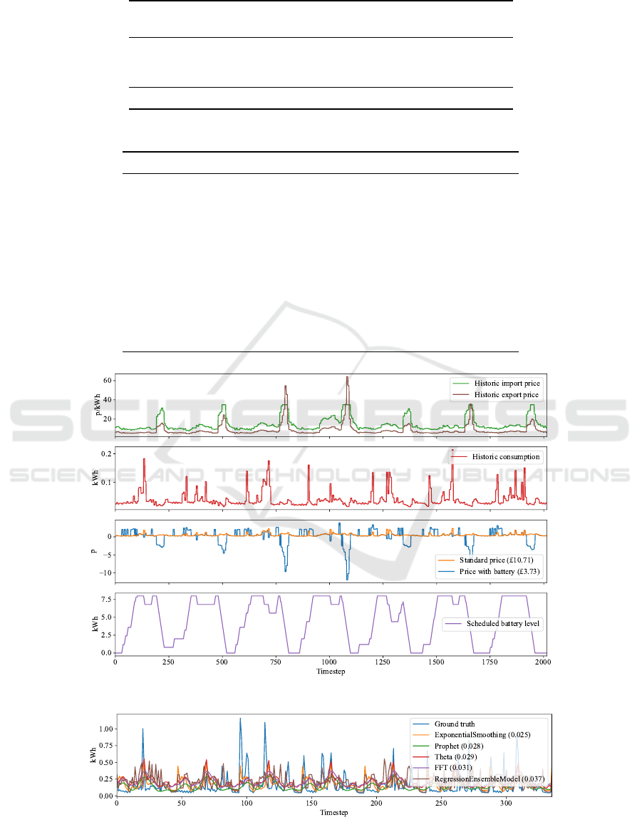
Table 1: Consumption and price forecasts for Example 1.

t U(t) P

(t) P

(t) U(t)

(t)

+U(t)

−

(t)

∗

(t)

1 2.96 kWh 20.83p/kWh 15.64p/kWh 61.66p 14.79

2 −0.23 kWh 22.68p/kWh 18.35p/kWh −5.22p −45.51

3 0.19 kWh 25.62p/kWh 20.29p/kWh 4.87p −41.8

Σ 2.92 kWh 69.13p/kWh 54.28p/kWh 61.31p −72.52

Table 2: Applicable battery schedules for Example 1.

i π

∀t ∈ D,C(s

,t, π

) V (s

,1,π

) Price

1 (−1, 0, −1) (0.0, 40.29, 0.0) 40.29 −32.22p

2 (−1, −1, 0) (0.0, 0.0, 46.67) 46.67 −25.85p

3 (0, −1, −1) (46.87, 0.0, 0.0) 46.87 −25.65p

4 (−1, 0, 0) (0.0, 40.29, 46.67) 86.96 14.44p

5 (0, 0, −1) (46.87, 40.29, 0.0) 87.16 14.64p

6 (−1, 1, −1) (0.0, 91.32, 0.0) 91.32 18.81p

7 (0, −1, 0) (46.87, 0.0, 46.67) 93.53 21.02p

8 (−1, −1, 1) (0.0, 0.0, 104.31) 104.31 31.79p

9 (0, 0, 0) (46.87, 40.29, 46.67) 133.82 61.31p

10 (−1, 1, 0) (0.0, 91.32, 46.67) 137.99 65.47p

11 (−1, 0, 1) (0.0, 40.29, 104.31) 144.6 72.09p

12 (0, −1, 1) (46.87, 0.0, 104.31) 151.18 78.66p

Figure 1: Battery scheduling problem and optimal solution for Example 2.

Figure 2: Consumption predictions for Example 4 with MSE in brackets.

A Smart Home Testbed for Evaluating XAI with Non-experts

777

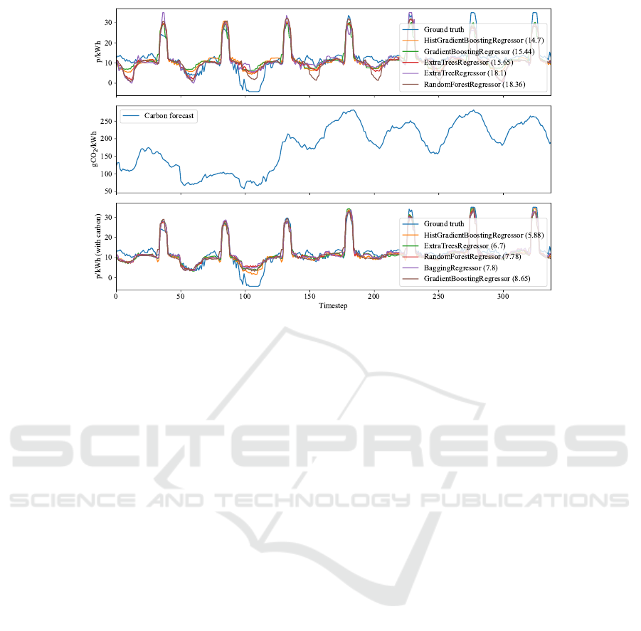
Figure 3: Import price predictions for Example 3 with MSE in brackets.

features to encode time (month, day, day-of-week,

hour, and minute). The ﬁrst plot in Figure 3 shows the

top performing regressors according to mean squared

error (MSE), with Histogram-based Gradient Boost-

ing Regression Tree achieving best performance. The

second plot then shows carbon forecast data for the

same period. Finally, the third plot shows improved

results where carbon forecast is included as an addi-

tional feature, with the best performing regressor see-

ing a reduction in MSE from 14.7 to 5.88.

3.1.3 Predicting Electricity Consumption

The simple approach described in Section 3.1.2 can

produce reasonable predictions in many cases. How-

ever, there are also techniques designed speciﬁcally

for time series data, known as time series forecast-

ing (Hyndman and Athanasopoulos, 2018). Suitable

models can thus be learned in practice using dedicated

tools for time series forecasting such as Darts (Herzen

et al., 2021) or sktime (L

oning et al., 2019). These

techniques are typically better than general-purpose

machine learning techniques at handling time-related

patterns such as seasonality, which may be impor-

tant if/when additional features are not readily avail-

able (as may be the case for predicting domestic elec-

tricity consumption). Nonetheless, many time series

forecasting techniques also support inclusion of addi-

tional features (called multivariate time series).

Example 4. Figure 2 shows consumption predictions

using standard regressors from Darts. Models were

trained on author-collected consumption data for the

period from 10 February 2021 to 25 July 2021, inclu-

sive, with the ﬁnal 7 days (336 timesteps) reserved for

validation. The only two features are timestamps and

consumption. Unless stated otherwise, seasonality is

set as 1-day (48 timesteps) for all applicable models.

The plot in Figure 2 shows the top performing regres-

sors according to MSE, with Exponential Smoothing

achieving best performance. Note that the ensemble

model is based on a random forest over two Naive

Seasonal models (using 1-day and 7-day seasonality).

3.2 Smart TRV

Smart home heating systems are a major category in

the smart home domain (Guo et al., 2019). Success-

ful commercial products include the ecobee range and

the previously mentioned Nest Learning Thermostat.

The AI literature has also seen many relevant appli-

cations (e.g. Rogers et al., 2013; Yang and Newman,

2013; Shann et al., 2017). Typical AI-based features

include the optimisation of heating controls according

to some criteria (e.g. comfort, cost, carbon emissions)

and the ability to automatically learn a heating sched-

ule. Perhaps the most high-proﬁle class of applica-

tion is smart thermostats, which connect directly to

a main heating system (e.g. boiler) and provide cen-

tralised control. Another class of application is smart

TRVs, which connect to a radiator and are limited

to localised (e.g. room-level) control. The same AI-

based features are applicable in either case.

We now introduce our second application, which

is centred on scheduling a smart TRV to optimise

comfort with respect to a learned heating schedule,

similar to the above applications. Smart TRVs are

ICAART 2022 - 14th International Conference on Agents and Artiﬁcial Intelligence

778

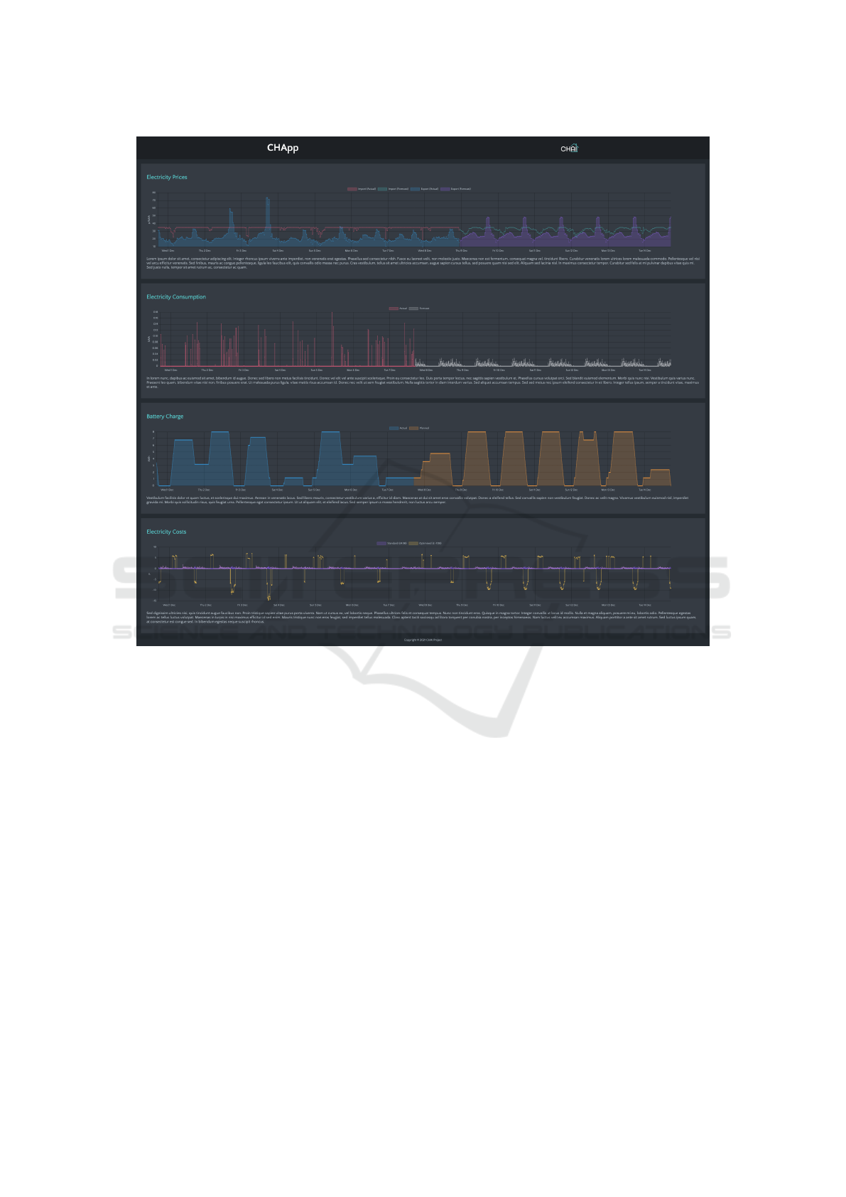
Figure 4: Sample page from user interface.

chosen as a low-cost alternative to smart thermostats

that are easier to install in homes for short-term evalu-

ations. Nonetheless, the application can easily extend

to the use of smart thermostats when practical. Again

the control schedule is deﬁned for some ﬁxed period

into the future (e.g. one week). Obvious issues in-

clude the building of a realistic thermal model and the

need to automatically elicit user heating preferences.

Generating the heating schedule presents avenues for

the use of machine learning, while optimal schedul-

ing of TRV actions presents avenues for the use of AI

planning. The application is a hybrid-AI system. Tar-

get XAI stakeholders are non-experts occupying the

home, with explainable AI planning needed to explain

the control schedule, and explainable machine learn-

ing needed to explain the learned heating schedule.

3.2.1 Scheduling TRV Control

Again we start by formalising the high-level AI plan-

ning problem as follows:

Deﬁnition 3. A TRV scheduling problem is a tuple

(τ,x

,σ, ω,λ,∆,t

max

,H) where:

• τ ∈ R

≥5

is the (constant) boiler temperature in °C

• x

∈ [5, τ] the (current) radiator temperature in °C

• y

∈ R is the (current) room temperature in °C

• σ ∈ R

≥0

is the BTU–50 gain in BTU/h

• ω ∈ R

≥0

is the BTU loss in BTU/h

• λ ∈ R

is the BTU effort in BTU/h

• ∆ ∈ R

is the number of timesteps per hour

• t

max

∈ N is the horizon with D = {1,2,.. .,t

max

}

• H : {t + 1 | t ∈ D} → R is the heating schedule

Deﬁnition 3 introduces parameters for our ther-

mal model, including properties of the heating system

and current environment. The heating schedule is de-

ﬁned for t = t

max

+ 1 but is undeﬁned for t = 1. Note

that BTU (British Thermal Unit) is a standard unit of

heat. The BTU–50 gain for a radiator is determined

by σ = e · a where e ∈ [0,1] is the radiator efﬁciency

A Smart Home Testbed for Evaluating XAI with Non-experts

779

and a ∈ R

≥0

is the radiator panel area in cm

. Stan-

dard efﬁciencies are: e = 0.55 for type 11 radiators

(single panel with no ﬁns), e = 0.77 for type 21 ra-

diators (single panel with ﬁns), and e = 1 for type

22 radiators (double panel with ﬁns). For example,

a type 11 radiator with a panel area of 3500 cm

has

a BTU–50 gain of σ = 3500 · 0.55 = 1925 BTU. As

in Deﬁnition 1 we assume that timesteps map to con-

secutive ﬁxed-length time intervals, although interval

length is now explicitly encoded by ∆. For example,

if ∆ = 12 then timesteps map to 5-minute intervals.

Deﬁnition 4. Let (τ,x

,σ, ω,λ,∆,t

max

,H) be a

TRV scheduling problem. A TRV scheduling model

is an MDP (S,A, T,C,t

max

) where:

• S = R

is the set of states with (x,y) ∈ S such that

x is the radiator temperature and y is the room

temperature

• A = {0,1} is the set of (TRV) actions with 1 the

valve open action and 0 the valve closed action

• T : S ×A → S is the transition function deﬁned for

each s ∈ S and each a ∈ A as:

= min{τ,max{5, x

}} (8)

(

x +

12(τ−x)

∆

if a = 1

max{y

,x +

4(y−τ)

∆

} if a = 0

(9)

= y +

(a · σ · β) − ω

λ · ∆

(10)

β = 0.000112378 · z

+ 0.0143811 · z (11)

where s = (x,y), z = x − y, and T (s,a) = (x

)

• C : S × D → R

≥0

is the cost function deﬁned for

each s ∈ S and each t ∈ D as:

C(s,t, a,s

) = |y

− H(t + 1)| (12)

where s

= (x

)

• t

max

∈ N is the horizon with D = {1,2,.. .,t

max

}

• s

∈ S is the initial state with s

= (x

)

Equations 8–11 deﬁne a simple building thermal

model (Bacher and Madsen, 2011) similar to Rogers

et al. (2011, 2013). We can summarise the model as

follows. Equation 9 says that when the TRV is open

the radiator takes 5 minutes (

/∆) to reach boiler tem-

perature, and when the TRV is closed takes 15 min-

utes (

/∆) to reach room temperature. Equation 8 en-

sures that radiator temperature is bounded by [5,τ].

Equation 11 is a standard calculation of radiator BTU

with respect to room temperature. Equation 10 de-

ﬁnes the change in room temperature with respect to

radiator BTU gain and room heat loss. For cost func-

tion C, Equation 12 deﬁnes cost at timestep t ∈ D as

the absolute deviation at t between the expected room

temperature and heating schedule. Therefore, C is

Figure 5: TRV problem and optimal solution for Example 5.

guaranteed to be non-negative. Note that Equation 1

can be adapted to this setting by replacing C(s,a) with

C(s,t, a,s

). An (optimal) TRV schedule is an (opti-

mal) partial policy that is closed with respect to s

∈ S.

Example 5. Let τ = 60 °C, x

= y

= 18 °C, σ = 1925

BTU/h, ω = λ = 500 BTU/h, ∆ = 4, t

max

= 24, i.e.

timesteps map to 15-minute intervals and a period of

6 hours. Figure 5 then shows a heating schedule H

with expected room (resp. radiator) temperature while

executing the optimal TRV schedule shown in the ﬁrst

(resp. second) plot, i.e. the TRV is open (resp. closed)

when the radiator temperature is increasing (resp. de-

creasing) or at boiler (resp. room) temperature.

TRV scheduling problems exhibit similar proper-

ties as battery scheduling problems: they cannot be

expressed (compactly) in standard AI planning lan-

guages, but non-negative costs mean they can still be

solved by standard search algorithms. The main dif-

ference for state-space search is that TRV scheduling

problems exhibit a much larger set of reachable states

due to more complex dynamics. In practice, unin-

formed search algorithms such as uniform cost search

can still ﬁnd solutions, but in order to scale to larger

decision horizons more advanced heuristic search al-

gorithms may be required. This highlights the need

for a broad range of explainable AI planning meth-

ods, e.g. uninformed strategies may be more intuitive

(and thus easier to explain) than heuristic strategies.

3.2.2 Learning Heating Preferences

Several commercial products use machine learning to

learn heating preferences (setpoint schedules), such as

the Auto-Schedule feature of the Nest Learning Ther-

mostat or the eco+ feature of the ecobee range, yet

the actual methods in use remain trade secrets (Bar-

rett and Linder, 2015). To the best of our knowledge,

the problem has not received much attention in the AI

literature, although there are some examples (e.g. Bao

and Chung, 2018). Unlike the machine learning prob-

lems described in Sections 3.1.2 and 3.1.3, learning

a user heating schedule H does not exhibit a crisply

ICAART 2022 - 14th International Conference on Agents and Artiﬁcial Intelligence

780

deﬁned scope or range of applicable machine learn-

ing techniques. Conceptually, the problem can be

conceived as an instance of a broader problem that

we refer to as learning from expert input. Essen-

tially the learned schedule represents a model of the

user’s heating preferences, with manual setpoint ad-

justments implying that the current model should be

revised, and an absence of manual adjustments im-

plying support for the current model. Initially the

system may rely entirely on manual adjustments (e.g.

the Nest begins to adopt learned setpoints from day

two)

but over time should require fewer manual ad-

justments as more data is acquired. However, research

studies have found users unsatisﬁed with schedules

learned by existing commercial systems (Yang and

Newman, 2013), which highlights the difﬁculties in

inferring user preferences from limited data.

The general problem of learning from expert input

can be solved by a potentially vast range of machine

learning techniques. Perhaps most relevant is a topic

that Russell and Norvig (2020, Chapter 22) refer to

as apprenticeship learning. This topic is said to in-

clude both imitation learning (Hussein et al., 2017)

and inverse reinforcement learning (Arora and Doshi,

2021). While reinforcement learning seeks to learn

a good policy (mapping states to actions) given ob-

served rewards, inverse reinforcement learning seeks

to learn a reward function given observed state-action

pairs. Conversely, imitation learning uses supervised

learning on observed state-action pairs in order to (di-

rectly) learn a policy that mimics observed behaviour.

In practice inverse reinforcement learning may be

more robust than imitation learning, since it learns ex-

pert preferences explicitly, but we speculate that com-

mercial smart thermostats in fact use imitation learn-

ing to learn user heating schedules. There are no com-

prehensive software libraries for apprenticeship learn-

ing akin to Scikit-learn or Darts, but collected imple-

mentations of selected methods are available.

4 TESTBED

This section describes technical details relevant to de-

ployment of our testbed (referred to here as CHApp).

4.1 Software Architecture

Figure 6 provides an overview of the software archi-

tecture, which is comprised of ﬁve components. The

ﬁrst (chapp-ui) is a web-based user interface imple-

https://support.google.com/googlenest/answer/

9247510

https://github.com/HumanCompatibleAI/imitation

chapp-api

Python

Falcon

Bjoern

chapp-service

Python

Schedule

Scikit-learn

Darts

chapp-ui

HTML

CSS (Flexbox)

JavaScript

Chart.js

SQLite

chapp-setup

Debian

Bash

Nginx

HTTP

Python

Browser

Python

Figure 6: Software architecture.

mented using standard web languages (HTML, CSS,

JavaScript) with the CSS Flexible Box Layout used

for compatibility on mobile devices (responsive web

design) and the Chart.js library used for dynamic data

visualisation. The second is an SQLite database used

for data persistence, storing all relevant data (e.g.

prices, consumption, predictions, schedules). The

third (chapp-api) is a JSON-based web API that ex-

poses data to the web interface and is implemented

in Python using the Falcon and Bjoern libraries. The

fourth (chapp-service) is a software service that is re-

sponsible for maintaining the database and providing

all AI functionality; it is implemented in Python using

the previously mentioned Scikit-learn and Darts li-

braries with the Schedule library used to execute reg-

ular tasks (e.g. data updates, model updates). The ﬁfth

(chapp-setup) is a deployment script implemented in

Bash that automatically installs and conﬁgures the

testbed on any recent Debian-based operating system,

with the Nginx web server used for hosting the web

interface. The database will typically run on the same

machine as both chapp-service and chapp-api, but

chapp-ui may run on a separate machine. In practice

there may be two instances of chapp-{service, api},

one for each application (e.g. chapp-battery, chapp-

trv). All software can be accessed via chapp-setup.

4.2 Hardware

Baseline deployment of the smart home battery ap-

plication requires installation of a single embedded

computer (to run the testbed software) and a single

smart plug (to capture electricity consumption data).

Suitable embedded computers include the Nvidia Jet-

son Nano and the Raspberry Pi. A popular smart plug

is the Eve Energy, although it currently has no avail-

able API to access consumption data. Possible alter-

natives include the Meross range, which has an un-

ofﬁcial API.

Deployment can easily scale to the in-

stallation of multiple smart plugs, e.g. Meross data is

accessed via a centralised web service for all plugs

https://github.com/kevinmcareavey/chapp-setup

https://github.com/albertogeniola/MerossIot

A Smart Home Testbed for Evaluating XAI with Non-experts

781

registered to a given user account. If feasible, smart

meters of course provide a more accurate measure of

total home electricity consumption, and data can usu-

ally be accessed in a similar manner though ofﬁcial or

unofﬁcial APIs. Examples of smart home batteries in-

clude the previously mentioned Tesla Powerwall and

Powervault 3 range.

Baseline deployment of the smart TRV applica-

tion requires installation of a single embedded com-

puter (again to run the testbed software), a single

smart TRV (to physically open/close the valve and to

measure radiator temperature), and a single tempera-

ture sensor (to measure room temperature). Note that

consumer smart TRVs typically include an on-board

sensor to measure room temperature but proximity

to the radiator may lead to unreliable measurements.

Suitable TRVs include the Netatmo Smart Radiator

Valve and the Lightwave Smart Radiator Valve. Suit-

able temperature sensors include the Netatmo Smart

Indoor Module and the Bosch BME680. Netatmo

provides a uniﬁed API,

while separate APIs are

available for Lightwave

and Bosch

devices. As

mentioned previously, the smart TRV may be re-

placed by a smart thermostat when practical.

4.3 User Interface

The web-based user interface is the primary means

by which end-users interact with the testbed. Figure 4

provides a screenshot of a single page from chapp-

ui. The page is comprised of several charts covering a

period of ±7 days relative to the current time, includ-

ing both historic data and future projections. The ﬁrst

three charts show electricity prices, smart plug energy

consumption, and simulated battery levels, respec-

tively, while the fourth chart shows electricity costs

with and without use of the battery. All charts are dy-

namic; they automatically update when new data is

available, and are customisable by end-users (e.g. to

focus on import prices by hiding export prices).

The user interface component is crucial to XAI

in that it must implement any user-facing aspects of

XAI features. Researchers must therefore adapt this

component in order to support any new XAI tools and

methods under evaluation. The software architecture

described in Section 4.1 is intended to ease this pro-

cess. For example, chapp-api provides a standard API

to access data, which means that e.g. chapp-ui can be

replaced by an alternative web interface without the

need to integrate with (or understand) the underlying

https://dev.netatmo.com/apidocumentation

https://support.lightwaverf.com/hc/en-us/articles/

360020665652-Link-Plus-Smart-Series-API-

https://circuitpython.readthedocs.io/projects/bme680

database. For some research studies a dedicated mo-

bile app may be preferable, in which case the app can

integrate with the testbed via chapp-api as usual.

5 RELATED WORK

Most similar to our applications are three strands

of research involving the University of Southampton

and University of Zurich. The ﬁrst strand consid-

ers smart thermostats that learn a building thermal

model (Rogers et al., 2011, 2013). The second consid-

ers smart thermostats that balance trade-offs between

comfort and electricity costs (Shann and Seuken,

2013, 2014; Alan et al., 2016b; Shann et al., 2017).

The third considers software agents that monitor elec-

tricity consumption and subsequently help users to se-

lect among daily electricity tariffs (Alan et al., 2014,

2015, 2016a). Obvious similarities include the use of

a thermal model for heating control (Section 3.2.1),

optimising electricity costs (Section 3.1.1), and pre-

dicting electricity consumption (Section 3.1.3). These

similarities are by design; we have sought to develop a

general XAI testbed that mimics functionality and AI

technology that non-experts are likely to encounter.

Despite these similarities, however, there are also sev-

eral key differences. Firstly, we do not assume that

heating systems are powered by electricity. Although

the situation varies greatly across Europe, 87% of

homes in the UK are currently powered by gas com-

pared to 7% by electricity.

Secondly, and as a con-

sequence of the ﬁrst, we do not attempt to optimise

energy costs during heating control. Gas tariffs are

typically ﬁxed for customers, so the idea of optimis-

ing energy costs is less applicable. We do however

incorporate the idea of optimising electricity costs by

the introduction of a smart home battery.

6 CONCLUSION

In this paper we have proposed a general smart home

testbed intended to support research studies evaluat-

ing XAI with non-experts. The testbed is represen-

tative of leading smart home applications, supports a

range of AI tools in a modular fashion, and can be

easily deployed with the provided software architec-

ture using inexpensive consumer hardware. There are

several aspects in which the two testbed applications

as deﬁned could be further extended:

https://www.statista.com/statistics/426988/united-

kingdom-uk-heating-methods/

ICAART 2022 - 14th International Conference on Agents and Artiﬁcial Intelligence

782

Improved Dynamics: The AI planning models can

be easily adapted to support more realistic dynam-

ics. For the smart home battery, these might in-

clude asymmetric charge/discharge rates or a de-

cline in battery efﬁciency at certain levels (e.g.

above 85% and below 15% capacity). For the

smart TRV, these might include the impact of ex-

ternal temperature and weather conditions. Un-

certainty in dynamics can be dealt with in the

standard way (e.g. by replacing the determinis-

tic transition function with a stochastic transition

function), although this will lead to the setting

of planning under uncertainty. In the latter case,

schedules can be found using e.g. determinisa-

tion (Little and Thi

ebaux, 2007) or conformant

planning (Domshlak and Hoffmann, 2006).

Learned Dynamics: Dynamics of a real smart home

battery or heating system can be easily learned

as a stochastic transition function and then in-

crementally improved online based on real-world

performance, although the above considerations

apply in regards to planning under uncertainty.

Improved Learning: Section 3.1.2, Section 3.1.3,

and Section 3.2.2 demonstrate a range of applica-

ble machine learning techniques but there is scope

to improve the performance of machine learning

components, including via model optimisations,

alternative models, and additional data sources.

For the purpose of XAI research, however, perfor-

mance remains a secondary objective, and models

should be chosen with primary consideration to

the types of XAI under evaluation.

Our testbed will form the basis of a research study

scheduled for 2023 with prior end-user testing sched-

uled for 2022. The study will evaluate XAI with non-

experts as part of a broader study on the impact of AI

threats (Pitropakis et al., 2019); XAI is regarded here

as an important tool in enabling non-experts to detect

AI threats. The study will involve 20 homes selected

from the social housing sector in England, with par-

ticipants expected to cover a broad demographic.

ACKNOWLEDGEMENTS

This work received funding from the EPSRC CHAI

project (EP/T026820/1). The authors thank Hsueh-Ju

Chen for advice on smart TRV hardware, and Ryan

McConville for advice on machine learning aspects.

REFERENCES

Abdul, A., Vermeulen, J., Wang, D., Lim, B. Y., and

Kankanhalli, M. (2018). Trends and trajectories for

explainable, accountable and intelligible systems: An

HCI research agenda. In Proceedings of the 2018

Conference on Human Factors in Computing Systems

(CHI’18), pages 1–18.

Adadi, A. and Berrada, M. (2018). Peeking inside the

black-box: a survey on explainable artiﬁcial intelli-

gence (XAI). IEEE Access, 6:52138–52160.

Alan, A., Costanza, E., Fischer, J., Ramchurn, S., Rod-

den, T., and Jennings, N. R. (2014). A ﬁeld study of

human-agent interaction for electricity tariff switch-

ing. In Proceedings of the 13th International Confer-

ence on Autonomous Agents and Multiagent Systems

(AAMAS’14), pages 965–972.

Alan, A. T., Costanza, E., Ramchurn, S. D., Fischer, J.,

Rodden, T., and Jennings, N. R. (2016a). Tariff agent:

interacting with a future smart energy system at home.

ACM Transactions on Computer-Human Interaction,

23(4):1–28.

Alan, A. T., Ramchurn, S. D., Rodden, T., Costanza, E.,

Fischer, J., and Jennings, N. R. (2015). Managing en-

ergy tariffs with agents: a ﬁeld study of a future smart

energy system at home. In Adjunct Proceedings of the

2015 ACM International Joint Conference on Perva-

sive and Ubiquitous Computing and Proceedings of

the 2015 ACM International Symposium on Wearable

Computers (UbiComp-ISWC’15), pages 1551–1558.

Alan, A. T., Shann, M., Costanza, E., Ramchurn, S. D., and

Seuken, S. (2016b). It is too hot: An in-situ study of

three designs for heating. In Proceedings of the 2016

Conference on Human Factors in Computing Systems

(CHI’16), pages 5262–5273.

Anjomshoae, S., Najjar, A., Calvaresi, D., and Fr

amling,

K. (2019). Explainable agents and robots: Results

from a systematic literature review. In Proceedings

of the 18th International Conference on Autonomous

Agents and Multiagent Systems (AAMAS’19), pages

1078–1088.

Arora, S. and Doshi, P. (2021). A survey of inverse

reinforcement learning: Challenges, methods and

progress. Artiﬁcial Intelligence, 297:103500.

Arrieta, A. B. et al. (2020). Explainable artiﬁcial intel-

ligence (XAI): Concepts, taxonomies, opportunities

and challenges toward responsible AI. Information

Fusion, 58:82–115.

Bacher, P. and Madsen, H. (2011). Identifying suitable

models for the heat dynamics of buildings. Energy

and Buildings, 43(7):1511–1522.

Bao, N. and Chung, S.-T. (2018). A rule-based smart ther-

mostat. In Proceedings of the 2018 International Con-

ference on Computational Intelligence and Intelligent

Systems (CIIS’18), pages 20–25.

Barrett, E. and Linder, S. (2015). Autonomous HVAC con-

trol, a reinforcement learning approach. In Proceed-

ings of the European Conference on Machine Learn-

ing and Principles and Practice of Knowledge Discov-

ery in Databases (ECML-PKDD’15), pages 3–19.

A Smart Home Testbed for Evaluating XAI with Non-experts

783

Biran, O. and Cotton, C. (2017). Explanation and justiﬁca-

tion in machine learning: A survey. In Proceedings of

the IJCAI’17 Workshop on Explainable Artiﬁcial In-

telligence (XAI’17), pages 8–13.

Chakraborti, T., Sreedharan, S., and Kambhampati, S.

(2020). The emerging landscape of explainable auto-

mated planning & decision making. In Proceedings of

the 29th International Joint Conference on Artiﬁcial

Intelligence (IJCAI’20), pages 4803–4811.

Cheng, H.-F. et al. (2019). Explaining decision-making

algorithms through UI: Strategies to help non-expert

stakeholders. In Proceedings of the 2019 CHI Con-

ference on Human Factors in Computing Systems

(CHI’19), pages 1–12.

Domshlak, C. and Hoffmann, J. (2006). Fast probabilistic

planning through weighted model counting. In Pro-

ceedings of the 16th International Conference on Au-

tomated Planning and Scheduling (ICAPS’06), pages

243–252.

Geffner, H. and Bonet, B. (2013). A Concise Introduction to

Models and Methods for Automated Planning. Mor-

gan & Claypool Publishers.

Guo, X., Shen, Z., Zhang, Y., and Wu, T. (2019). Review

on the application of artiﬁcial intelligence in smart

homes. Smart Cities, 2(3):402–420.

Herzen, J. et al. (2021). Darts: User-friendly modern ma-

chine learning for time series. arXiv:2110.03224.

Hoffman, R. R., Mueller, S. T., Klein, G., and Litman, J.

(2018). Metrics for explainable AI: Challenges and

prospects. arXiv:1812.04608.

Hussein, A., Gaber, M. M., Elyan, E., and Jayne, C. (2017).

Imitation learning: A survey of learning methods.

ACM Computing Surveys, 50(2):21.

Hyndman, R. J. and Athanasopoulos, G. (2018). Forecast-

ing: principles and practice. OTexts, 2nd edition.

Kraus, S. et al. (2020). AI for explaining decisions in multi-

agent environments. In Proceedings of the AAAI Con-

ference on Artiﬁcial Intelligence (AAAI’20), pages

13534–13538.

Langer, M. et al. (2021). What do we want from explain-

able artiﬁcial intelligence (XAI)?–a stakeholder per-

spective on XAI and a conceptual model guiding in-

terdisciplinary XAI research. Artiﬁcial Intelligence,

296:103473.

Lipton, Z. C. (2018). The mythos of model interpretability:

In machine learning, the concept of interpretability is

both important and slippery. ACM Queue, 16(3):31–

57.

Little, I. and Thi

ebaux, S. (2007). Probabilistic planning vs.

replanning. In Proceedings of the ICAPS Workshop on

Planning Competitions: Past, Present, and Future.

oning, M., Bagnall, A., Ganesh, S., Kazakov, V., Lines, J.,

and Kir

aly, F. J. (2019). sktime: A uniﬁed interface

for machine learning with time series. In Proceed-

ings of the NeurIPS Workshop on Systems for Machine

Learning.

Mekuria, D. N., Sernani, P., Falcionelli, N., and Dragoni,

A. F. (2019). Smart home reasoning systems: a sys-

tematic literature review. Journal of Ambient Intelli-

gence and Humanized Computing, pages 1–18.

Miller, T. (2019). Explanation in artiﬁcial intelligence: In-

sights from the social sciences. Artiﬁcial Intelligence,

267:1–38.

Pedregosa, F. et al. (2011). Scikit-learn: Machine learning

in Python. Journal of Machine Learning Research,

12:2825–2830.

Pitropakis, N., Panaousis, E., Giannetsos, T., Anastasiadis,

E., and Loukas, G. (2019). A taxonomy and survey of

attacks against machine learning. Computer Science

Review, 34:100199.

Rogers, A., Ghosh, S., Wilcock, R., and Jennings, N. R.

(2013). A scalable low-cost solution to provide per-

sonalised home heating advice to households. In

Proceedings of the 5th ACM Workshop on Embedded

Systems For Energy-Efﬁcient Buildings (BuildSys’13),

pages 1–8.

Rogers, A., Maleki, S., Ghosh, S., and Jennings, N. R.

(2011). Adaptive home heating control through

gaussian process prediction and mathematical pro-

gramming. In Proceedings of the 2nd International

Workshop on Agent Technology for Energy Systems

(ATES’11).

Russell, S. J. and Norvig, P. (2020). Artiﬁcial Intelligence:

A Modern Approach. Prentice Hall, 4th edition.

Shann, M., Alan, A., Seuken, S., Costanza, E., and Ram-

churn, S. D. (2017). Save money or feel cozy?: A

ﬁeld experiment evaluation of a smart thermostat that

learns heating preferences. In Proceedings of the 16th

Conference on Autonomous Agents and Multiagent

Systems (AAMAS’17), pages 1008–1016.

Shann, M. and Seuken, S. (2013). An active learning ap-

proach to home heating in the smart grid. In Proceed-

ings of the 23rd International Joint Conference on Ar-

tiﬁcial Intelligence (IJCAI’13), pages 2892–2899.

Shann, M. and Seuken, S. (2014). Adaptive home heat-

ing under weather and price uncertainty using gps and

mdps. In Proceedings of the 13th International Con-

ference on Autonomous Agents and Multiagent Sys-

tems (AAMAS’14), pages 821–828.

Yang, R. and Newman, M. W. (2013). Learning from a

learning thermostat: lessons for intelligent systems for

the home. In Proceedings of the 2013 ACM Interna-

tional Joint Conference on Pervasive and Ubiquitous

Computing (UbiComp’13), pages 93–102.

ICAART 2022 - 14th International Conference on Agents and Artiﬁcial Intelligence

784