Forecasting Extractions in a Closed Loop Supply Chain of Spare Parts:

An Industrial Case Study

Emna Turki

1,3 a

, Oualid Jouini

1 b

, Ziad Jemai

2 c

, Laura Urie

, Adnane Lazrak

, Patrick Valot

and

Robert Heidsieck

Laboratoire Genie Industriel, CentraleSup

elec, Universit

e Paris-Saclay, 3 rue Joliot-Curie, 91190 Gif-sur-Yvette, France

Laboratoire OASIS,

Ecole Nationale d’Ing

enieurs de Tunis, Universit

e Tunis El Manar, BP37, 1002 Tunis, Tunisia

General Electric Healthcare, 283 Rue de la Mini

ere, 78530 Buc, France

robert.heidsieck@med.ge.com

Keywords:

Healthcare Industry, Closed Loop Supply Chain, Spare Parts Harvesting, Intermittent Demand Forecasting.

Abstract:

In healthcare industry, companies like GEHC (General Electric Healthcare) buy back their products at the EOL

(End of Life) phase and reuse the spare parts composing them. This process is referred to as spare parts har-

vesting. The harvested parts are included in the spare parts supply chain which presents speciﬁc characteristics

like the availability of critical parts and the intermittent demand behavior. Add to that, the unpredictability

of the parts’ supply capacity from bought back systems is a challenge for healthcare companies. The focus

of this paper is to provide an accurate forecasting method of the harvested parts supply capacity for GEHC.

To achieve this objective, a comparative study is carried out between statistical forecasting models. Then, a

forecasting process employing the most accurate models is provided using TSB-Croston, the 12-month mov-

ing average, the best ARIMA model chosen with the Box-Jenkins methodology, and an introduced business

knowledge based model. In order to improve the designed method accuracy, the statistical models’ forecast is

adjusted using contextual information. An error measurement based on a modiﬁed MAPE error is introduced

to evaluate the forecast. By means of the designed method, the monthly accuracy is improved by 9%.

1 INTRODUCTION

Closed loop supply chain continues to receive aca-

demic and managerial interest thanks to its efﬁciency

to limit wastes, to allow additional proﬁts, and to re-

spect service contracts. At the EOL phases of the

products, it is difﬁcult to maintain the same quality

of service for customers. Given that the production

of spare parts decreases at these stages, other options

can be considered to manage the spare parts supply

chain. One of the options is the buyback of products

and the reuse of parts composing them. This process

is referred to as spare parts harvesting. In Healthcare

industry, companies like GEHC buy back their health-

care systems and they either sell them with a lower

price or reuse the parts. Before being stocked, har-

vested parts are subject to a quality control process

in order to guarantee a similar quality to new parts.

However, the quantity of parts extracted from these

https://orcid.org/0000-0002-7002-7722

https://orcid.org/0000-0002-9498-165X

https://orcid.org/0000-0001-7679-9670

systems is unpredictable. Furthermore, extractions’

lead-times can differ depending on numerous factors

like the part’s type and the system’s condition. There-

fore, accurate spare parts supply capacity forecasting

methods need to be implemented. This reverse supply

chain presents a high complexity due to several ele-

ments like inventory limitations, intermittent demand

behavior, and parts characteristics. Further inﬂuenc-

ing features on the parts’ availability are the IB (In-

stalled Base) size and the frequency of the systems’

buyback. These features are referred to as contex-

tual information that help developing spare parts fore-

casting methods relying not only on statistical models

but also on additional ﬁeld information (Pinc¸e et al.,

2021).

In previous works, the use of statistical forecasting

methods and contextual information aimed at predict-

ing the clients’ consumption of spare parts (Mathews

and Diamantopoulos, 1986, 1992). The supplied parts

from reused systems have not been investigated and

looked at as an important information to predict.

In this paper, a business knowledge based fore-

236

Turki, E., Jouini, O., Jemai, Z., Urie, L., Lazrak, A., Valot, P. and Heidsieck, R.

Forecasting Extractions in a Closed Loop Supply Chain of Spare Parts: An Industrial Case Study.

DOI: 10.5220/0010906700003117

In Proceedings of the 11th International Conference on Operations Research and Enterprise Systems (ICORES 2022), pages 236-243

ISBN: 978-989-758-548-7; ISSN: 2184-4372

casting model using the parts extraction history and

contextual information is introduced. Existing statis-

tical models along with the introduced model are ap-

plied on more than 1300 time series with intermittent

behavior representing GEHC spare parts harvesting

history. A modiﬁcation of the MAPE error is applied

to make it suitable for the intermittent behavior of

parts extractions. The application process of the most

ﬁtted model for each time series is then presented. Fi-

nally, the results of the designed method are discussed

and further research suggestions are provided.

2 LITERATURE REVIEW

Time series forecasting has been widely applied, not

only in academic circles, but also in different indus-

tries and businesses over the last decades. It aims to

collect, to analyze the past observations, and to de-

velop an appropriate model ﬁtted to the structure of

the series. Then, this model can be used to predict

future values (Ivanovski et al., 2018). However, the

application of the forecasting methods has been nar-

rowed to the spare parts clients’ demand mostly in

case of a one-way supply chain.

Some of the applied forecasting models are based

on a trivial logic of calculations like the Average, the

ıve and the Seasonal Na

ıve forecasts. Other mod-

els, a bit more complex yet simple, can be more ad-

equate to the data such as the MA (Moving Average)

which has a property to reduce the noise or the varia-

tion in time series. One of the extensively used mod-

els in demand forecasting is SES (Simple Exponential

Smoothing). It is considered as a statistically simple

model as it cannot deduce trend in data. Nevertheless,

in many occasions, it has outperformed the MA and

robust models (Makridakis and Hibon, 2000).

Another used method is ARIMA which is widely

employed thanks to the Box-Jenkins methodology

that helps identify the optimum parameters (Box

et al., 2015). The limitation of this model is the as-

sumption that there is a linear behavior in the time

series. Thus, non-linear patterns cannot be captured

(Zhang, 2003).

When it comes to sporadic, extremely variable de-

mand, the above models can perform poorly. This cat-

egory of demand is difﬁcult to predict and needs more

sophisticated calculations. J.D. Croston found that

intermittent demand often produces inappropriate in-

ventory levels and that forecasts of constant quantities

at ﬁxed intervals can double the inventory level of the

needed volumes (Croston, 1972). Therefore, a fore-

casting method that helps overcome the problems pro-

duced by intermittent demands was introduced. Nev-

ertheless, the major limitation of Croston’s model is

updating the forecasts only after a positive demand

occurrence which makes the model incompatible with

obsolescence problems (Teunter et al., 2011). Con-

sequently, Teunter, Syntetos and Babai proposed the

TSB-Croston method which updates its periodicity

estimate even if the demand does not occur (Xu

et al., 2012). They used the ME (Mean Error) to com-

pare between TSB-Croston and statistical models like

SES, Croston, and SBA and found that TSB-croston

was the most accurate (Teunter et al., 2011).

Such comparative studies of forecasting methods

have been exhaustively conducted in the purpose of

accurately forecasting intermittent demand. To fore-

cast aircraft spare parts demand, a research study

considered twenty methods and concluded that the

best ones are the moving averages, EWMA (Expo-

nentially Weighted Moving Average), and Croston’s

method (Regattieri et al., 2005). In the same domain,

a study was carried out comparing artiﬁcial intelli-

gence methods like the NN (Neural Network) and the

ABC classiﬁcation method with Croston, TSB Cros-

ton, SBJ Croston, MA, and SES, deduced that NN

with a high number of features outperforms the rest

of the methods (Amirkolaii et al., 2017). In another

paper, the Holt-Winters method and sARIMA perfor-

mances were investigated on a sporadic demand of

spare parts with seasonality and trend components. A

similar performance of the Holt-Winters method and

the best sARIMA was observed on the seasonal de-

mand patterns. However, when a trend component is

also present, sARIMA gave a better accuracy (Gam-

berini et al., 2010).

In the literature, demand forecasting improve-

ments are not only conducted by comparing the fore-

cast methods on the same set of data, but also by ex-

ploiting ﬁeld information and judgmental adjustments

of statistical models. In this regard, a research pa-

per studied the effect of judgmental adjustments made

by forecasters on a commercial statistical forecasting

system used by a pharmaceutical company to forecast

an intermittent demand. The authors concluded that

judgmentally adjusted forecast is more accurate than

the generated forecast by statistical models (Syntetos

et al., 2009). Although the role of judgment in fore-

casting is recognized by researchers and the interest in

this domain is increasing (Lawrence et al., 2006), re-

search works integrating contextual information and

statistical models in the intermittent demand forecast-

ing area are still limited (Pinc¸e et al., 2021).

When applying a demand forecasting model, the

probable occurrence of demand is estimated. In case

of time series forecasting, statistical models that can

differ depending on the demand pattern are exploited.

Forecasting Extractions in a Closed Loop Supply Chain of Spare Parts: An Industrial Case Study

237

Commonly applied models are generally not accurate

if the demand is not smooth. Therefore, it is important

to understand the demand pattern and to employ the

most suitable method (Eaves and Kingsman, 2004).

To categorize the demand into smooth, erratic, lumpy,

and intermittent, (Johnston and Boylan, 1996) cal-

culated the average inter-demand intervals. The au-

thors evaluated the suitability of Croston and expo-

nential smoothing models on different categories of

data using the MSE (Mean Squared error) with the

purpose of deﬁning the boundaries and then catego-

rizing the demand. They recommended that, if the av-

erage inter-demand interval is greater than 1.25, Cros-

ton’s method should be used and not the SES. Another

study was conducted on 3000 real-life intermittent de-

mand data from the automotive industry based on the

average inter-demand interval and the squared coefﬁ-

cient of demand variation. In this study, a demand

categorization scheme resulting from a comparison

between Croston and SBA-Croston was introduced

(Syntetos et al., 2005).

The evaluation of the forecasting models is em-

ployed using different error measurements with vari-

ous characteristics. The exhaustively used errors are

summarized in Table 1.

Table 1: The most used errors in literature.

Error measurement Formula

MAE

∑

i=1

− f

MSE

∑

i=1

− f

)

RMSE

√

MSE

Relative MAE

MAE

evaluated f orecastingmethod

MAE

naive f orecast

MASE q

−f

, b =

n−1

∑

− f

MAPE

100

∑

i=1

−f

sMAPE

2∗100

∑

i=1

−f

+ f

The application of these errors depends on their

suitability to the data and the needed performance

measurement. The MAE (Mean Absolute Error) mea-

sures prediction errors in the same unit as the orig-

inal series (Khair et al., 2017). The MSE (Mean

Squared Error) and RMSE (Root Mean Squared Er-

ror) are known for their theoretical relevance in sta-

tistical modelling (De Gooijer and Hyndman, 2006).

Yet, they are scale-dependant and more inﬂuenced

by outliers than the MAE (Hyndman and Koehler,

2006). The Relative MAE removes the scale of the

data by comparing the forecasts with those obtained

from a benchmark forecast model. The MASE er-

ror is a scale-free error which handles series with

inﬁnite values (Hyndman and Koehler, 2006). On

the other hand, the MAPE which is also a scale-free

error, cannot be used with values close to or equal

to zero (Wallach and Gofﬁnet, 1989). That’s why

the symmetric measures were proposed (Makridakis,

1993). Still, the value of sMAPE has a heavier penalty

with a higher forecast (Wallach and Gofﬁnet, 1989).

The choice of the error measurement is an important

step. That’s why the characteristics mentioned above

should be taken into account especially when com-

paring the forecast of several models on a sporadic

demand.

The efforts made in the domain of intermittent

demand forecasting are numerous. The forecasting

models’ application is mainly narrowed to the de-

mand forecasting area especially for spare parts. In

addition, existing methods employ statistical models

with limited attempts to include business knowledge

and judgmentally adjust the forecast.

A new methodology is presented in this paper

aiming to forecast the parts’ extraction capacity from

used systems. This new application area includes dif-

ferent elements like the IB, the number of bought back

systems, the extractions rate, the quality of parts, and

the inventory levels while the previous applications

mainly focused on the parts failure prediction. In ad-

dition, in demand forecasting, the studied pattern is

often related to a part’s failure in a system. Mean-

while, the main goal of this new methodology is to

predict the capacity to supply more than one part from

bought back systems.

This is achieved by providing a process to com-

pare between statistical models and an introduced

business based knowledge model allowing judgmen-

tal adjustments of predicted quantities.

3 PROBLEM SETTING

3.1 Problem Deﬁnition

To the traditional service parts new buy supply chain ,

the closed loop supply chain in GEHC offers two ad-

ditional supply solutions , the repair supply chain and

the parts’ harvesting supply chain. As the estimation

of repair supply chain volumes was already subject to

a previous research work (El Garrab et al., 2020), this

paper will focus on the harvest supply chain.

The choice between new parts, repaired parts, and

harvested parts from bought back systems depends on

several criteria like the lead-time, the parts criticality,

and the inventory levels of what has been provided

by each supplier. It can be taken by a management

system or manually. However, in either cases it is ap-

proved or declined by a team of planners. For this

team, the decision to use harvested parts is challeng-

ICORES 2022 - 11th International Conference on Operations Research and Enterprise Systems

238

ing considering that it can result in an overstock or a

shortage whenever the number of extracted parts ex-

ceeds or fails to reach the planned quantity.

Due to the intermittent behavior of harvested

parts, new buys are often preferred in order to satisfy

the customers’ needs even though they have higher

prices. Only frequently harvested parts are chosen if

they have shorter lead-times or in case the external

supplier is no longer an option.

Figure 1 illustrates the spare parts closed loop sup-

ply chain in which the parts are provided by one of the

three suppliers, stocked in a warehouse, and then dis-

tributed to maintain the IB. Unlike a one-way supply

chain, this supply chain presents a high complexity to

manage and to respect service contracts. Despite its

ﬁnancial beneﬁts and positive environmental impact,

the risk of being unable to satisfy the clients’ needs is

still high. For this reason, it is important to improve

this side of the supply chain visibility by providing an

accurate forecast of the harvested parts.

3.2 Data

With the aim of providing an accurate forecasting

method, a history of nearly 1300 harvested parts for

more than three years at GEHC is exploited. The goal

is to analyze the data behavior and to predict the fu-

ture extractions of parts using as much points as pos-

sible. The Syntetos et al. categorization scheme was

employed and it was found that 98% of the parts are

in the intermittent category and only 2% are in the

lumpy category (Syntetos et al., 2005).

Since the parts are grouped and shipped on a

monthly basis, a time series representing the total sum

of harvested parts is also analysed and a seasonality

component is detected. Mainly, the total extractions

quantity increased at the end of every quarter for the

ﬁrst two years. However, a change in the behavior due

to an inventory limitation is observed on the last two

years. The decision to harvest a part depends on this

limitation. In GEHC, the quantity of parts allowed to

be harvested corresponds to 24 months of the parts’

predicted consumption. This quantity was narrowed

down to 12 months consumption of parts in the 3rd

year of the studied period. That’s why, the harvested

quantity was reduced since then.

The total harvested parts seasonality and quantity

decrease are not clearly observed on each part’s his-

tory of extractions. That’s why, the same model can-

not be used for all parts and they need to be studied

separately in order to choose the most suitable one.

3.3 Forecasting Model

Several efforts were elaborated in the domain of in-

termittent demand forecasting. Some researchers ap-

plied time series models and others went for deep

learning models seeking to prove the efﬁciency of ar-

tiﬁcial intelligence in demand forecasting. Despite

that, the resulting methods are not yet proven to work

on every set of data. Hence, two different approaches

are applied in this research work and then evaluated

to choose the most ﬁtted model for each time series.

3.3.1 Approach 1

A forecast model based on the business knowledge is

developed. In this method, a capture rate of parts from

bought back systems is calculated as shown below:

CR% =

100 ×n

, (1)

where m is the number of bought back systems and n

is the number of parts extracted from them.

Due to the complexity of the studied supply chain,

several features like the inventory limitation, the sys-

tems volume, and the quantity of each part per system

may have an impact on the total extracted amount of

parts. Harvest center’s experts’ opinions were taken

into account and it was conﬁrmed that the inventory

limitation is the most impacting feature. This feature

is the decision to harvest or not the extracted part.

Namely, if a part is extracted, there is a possibility

that it cannot be harvested due to this decision. That’s

why, to predict the period it will take to change, the

inventory limitation is considered along with the stock

level of parts.

The forecast for a period of twelve months is cal-

culated as follows:

F =

CR% ×m

100

, (2)

where m’ is the number of expected systems buyback

for the next 12 months.

The forecast is then projected on the next twelve

months with respect to the inventory limitation. In

order to do that, two cases are distinguished:

• If the part’s harvesting is allowed: the forecast is

projected on the predicted period on which the de-

cision will not change. For the rest of the year, the

forecast is zero.

• If the part’s harvesting is not allowed: the forecast

is zero on the predicted period on which the deci-

sion will not change. For the rest of the year, the

forecast is calculated as follows:

Forecasting Extractions in a Closed Loop Supply Chain of Spare Parts: An Industrial Case Study

239

Figure 1: Spare parts closed loop supply chain.

F −

12 − p

, (3)

where f

is the forecast on month i, F is the total

predicted quantity, and p is the period on which

the harvesting decision will stay the same.

3.3.2 Approach 2

In this approach, four statistical models are tested and

compared with the aim of using the most accurate one

to forecast the spare parts supply capacity. The tested

models are MA, SES, Croston and TSB-Croston.

The models’ assessment on the harvested spare

parts is conducted using a modiﬁed MAPE error. In

case the actual and/or the predicted quantities are

equal to zero, the MAPE and the sMAPE give inﬁnite

values. Therefore, to make it suitable for the problem,

a change in the MAPE formula is indispensable . The

error is also caped at 100% in order to easily interpret

the results. The applied modiﬁcations are detailed in

the formula bellow:

Modiﬁed MAPE% = min(100,

100 ×|F −A|

max(A, 1)

) (4)

where A is the actual value of extracted parts and F is

the predicted values.

Using this error, TSB-Croston is chosen because it

outperforms the other models on 82% of the intermit-

tent parts category and 71% of the lumpy parts cate-

gory.

After three months of the forecast evaluation, an

underestimation of the predicted quantities is ob-

served. This is why ARIMA models are also con-

sidered and the Box-Jenkins method is used to iden-

tify the optimum parameters for each time series. The

forecast of these statistical models is adjusted by tak-

ing into consideration the inventory limitation and the

upcoming buyback of systems linked to the parts.

3.3.3 Forecast Process

After analyzing the results, Approach 1 is proven to

have a better ability to forecast the total volume of

parts since it relies on the products coming in the next

period and can predict zero quantities using the inven-

tory constraints for each part. However, on a monthly-

basis, Approach 2 outperforms Approach 1. For low

volume parts, TSB-Croston model is chosen as it is

able to be more accurate on intermittent demand and

to predict the interval of time between two demand

occurrences. For higher volume parts, ARIMA mod-

els are able to provide better results. At the same time,

the company’s current model which is a 12-month

MA (12-month Moving Average) is also able to per-

form a more accurate forecast than the proposed mod-

els on some parts.

These results led to think about an efﬁcient way

to perform the forecast using the best and most ﬁt-

ted model to the demand pattern on each part and

to evaluate both the predicted volume per period

(six to twelve months) and the quantity per month.

Therefore, a measurement of error called “Combined

MAPE” shown in equation 5 is introduced.

When evaluating the signiﬁcance of the monthly

and the volume modiﬁed MAPE errors, the company

experts conﬁrmed that it is as important to give an

accurate quantity on a twelve-month or a six-month

period as to forecast an accurate quantity per month

and prevent a part excess or obsolescence. As a

result, equal weights to each modiﬁed MAPE error

are set.

ICORES 2022 - 11th International Conference on Operations Research and Enterprise Systems

240

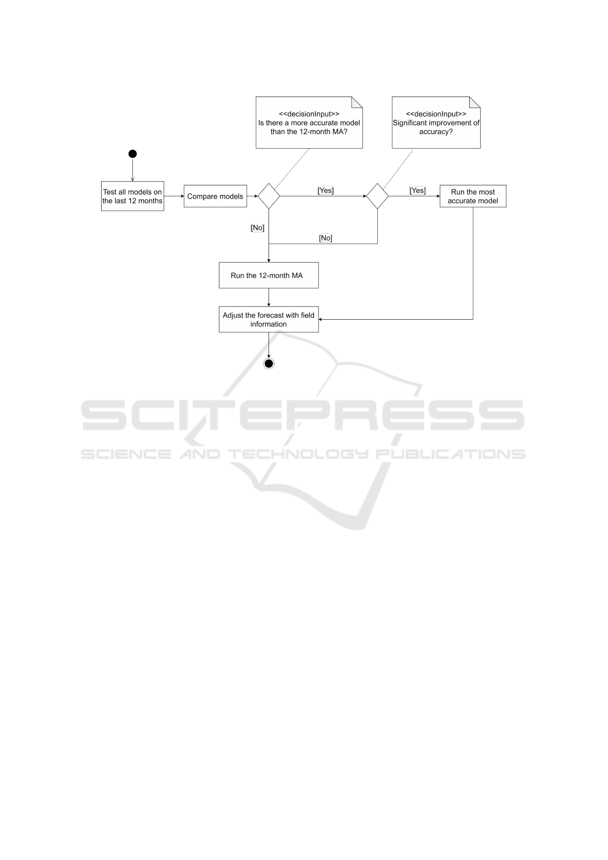
Figure 2: Forecast process for each spare part on month i.

Combined MAPE = 0.5 ×Volume modiﬁed MAPE

+ 0.5 ×Average Monthly modiﬁed MAPE (5)

The provided forecast overrides an existing forecast

computed by a commercial forecasting system em-

ploying a 12-month MA. For this reason, this model

is used as a benchmark method.

Only a signiﬁcant improvement in accuracy can

justify the forecast override. That’s why, an evalu-

ation of different scenarios if the override is applied

starting from a minimum improvement X in com-

bined accuracy was conducted and the chosen mini-

mum improvement in accuracy allowing to override

the forecast was X = 10%.

A process describing the steps needed to provide

the new forecast is illustrated in ﬁgure 2. To perform

the forecast on a part, the following steps are applied:

• The forecast of the next period using the chosen

models (TSB-Croston, 12-month MA, ARIMA,

and the business knowledge based model) is cal-

culated on month i.

• The models’ performances are evaluated using the

accuracy based on the combined MAPE. Then,

they are compared to the 12-month MA model.

• In case of a signiﬁcant improvement of accuracy

(improvement > 10 points), the most accurate

forecast model is chosen.

• The forecast is adjusted according to the inven-

tory limitation and the upcoming systems buy-

back linked to the part.

• Repeat the forecast steps in month i+1

4 RESULTS & DISCUSSION

To choose the best model for each part, two accu-

racy measurements are used on the entire population

of parts, then on a sample of parts with activity on a

given period. The purpose is to evaluate the ability of

the models to predict the actual extractions when they

occur and the right volume over a period of time.

The forecast performance on the ﬁrst six months

of implementation is assessed by means of an average

monthly accuracy and an average 6-month volume ac-

curacy for both samples.

The results can be inﬂuenced by various param-

eters. Different set of parameters allow to evaluate

different accuracy measurements and to have more

precise conclusions. Therefore, they are deﬁned as

follows:

• Population: P1 = Each month’s population/ P2 =

The entire population of parts.

• Activity: A1 ≥ 0 (all parts) / A2 ≥ 1 on period

Forecasting Extractions in a Closed Loop Supply Chain of Spare Parts: An Industrial Case Study

241

Table 2: Accuracy comparison of the designed method and the previously used model in GEHC.

Accuracy metric Parameters δ

accuracy

= Designed method

accuracy - 12-month MA accuracy

Avg. monthly accuracy over 6

months for all parts

P1, A1, I2, W1 +9%

Avg. 6-month volume accuracy for

all parts

P2, A1, I2, W2 +20%

Avg. monthly accuracy for parts

with activity on a 6-month period

P1, A2, I2, W2 +2%

Avg. 6-month volume accuracy for

parts with activity

P2, A2, I2, W2 +6%

• Improvement: I2 = parts with combined accuracy

improvement > 10 pts

• Accuracy window: W1 = 1 Month / W2 = 6

Months

An average monthly accuracy and an average 6-

month volume accuracy are calculated on the entire

population of parts and on the group of parts that had

at least one quantity over the test period. The results

are resumed in table 2.

Accuracy on all parts is improved by the designed

method. Compared to the previously used model in

GEHC which is a 12-month MA, improvements on

the volume accuracy are higher than the ones on the

monthly accuracy. Nevertheless, the volume accuracy

is always lower than the monthly accuracy. This result

can be explained by the fact that the studied period

contains two end of quarter months. Even though,

in the tested period a lower quantity of parts was ex-

tracted, the seasonality did not vanish. Since the used

statistical models do not consider seasonality, they

tend to adjust the forecast according to the latest pe-

riod. That’s why, the extracted quantities are under-

estimated. Therefore, the next step will be to evaluate

the suitability of ARIMA with seasonality to this data

set and to choose the best ﬁtted model for each part.

5 CONCLUSION &

PERSPECTIVES

The forecast models are applied to a scope of more

than 1300 references of parts within the closed loop

spare parts supply chain of GEHC. Choosing the most

ﬁtted model among the 12-month MA, the business

knowledge model, TSB-Croston and the best ARIMA

model chosen with the Box-Jenkins methodology and

adjusting the statistical forecast using ﬁeld informa-

tion delivered a better accuracy than the 12-month

MA model.

In GEHC, it was assumed that the quantity of har-

vested parts is the same for a rolling 12-month period.

That’s why, a 12-month MA was applied to estimate

the extracted quantity of parts each year. Nonetheless,

this supply chain is characterized by its complexity

and is inﬂuenced by various factors. For this reason,

it was important to add ﬁeld information to the pro-

posed forecast method and to consider the most im-

pacting features on the parts supply capacity.

Forecasting the parts extraction from bought back

systems accurately is an efﬁcient way to make this

side of the closed loop spare parts supply chain more

visible, to avoid the new buy of parts that can be har-

vested, and to improve customers’ satisfaction by pro-

viding parts in shorter lead-times.

In spite of the observed increase of the har-

vested spare parts supply capacity forecast accuracy,

more improvements should be applied to the statis-

tical models by adding the seasonality component to

ARIMA. Explicative models should also be evaluated

on this intermittent data. As AI solutions are imple-

mented in the domain of demand forecasting, they

should also be evaluated in the domain of reused parts

supply capacity forecasting.

REFERENCES

Amirkolaii, K. N., Baboli, A., Shahzad, M., and Tonadre,

R. (2017). Demand forecasting for irregular demands

in business aircraft spare parts supply chains by us-

ing artiﬁcial intelligence (ai). IFAC-PapersOnLine,

50(1):15221–15226.

Box, G. E., Jenkins, G. M., Reinsel, G. C., and Ljung, G. M.

(2015). Time series analysis: forecasting and control.

John Wiley & Sons.

Croston, J. D. (1972). Forecasting and stock control for

intermittent demands. Journal of the Operational Re-

search Society, 23(3):289–303.

De Gooijer, J. G. and Hyndman, R. J. (2006). 25 years of

time series forecasting. International journal of fore-

casting, 22(3):443–473.

Eaves, A. H. and Kingsman, B. G. (2004). Forecasting for

ICORES 2022 - 11th International Conference on Operations Research and Enterprise Systems

242

the ordering and stock-holding of spare parts. Journal

of the Operational Research Society, 55(4):431–437.

El Garrab, H., Castanier, B., Lemoine, D., Lazrak, A., and

Heidsieck, R. (2020). Towards hybrid machine learn-

ing models in decision support systems for predicting

the spare parts reverse ﬂow in a complex supply chain.

In Information system, Logistics & Supply Chain-ILS

2020, pages 188–195.

Gamberini, R., Lolli, F., Rimini, B., and Sgarbossa, F.

(2010). Forecasting of sporadic demand patterns with

seasonality and trend components: an empirical com-

parison between holt-winters and (s) arima methods.

Mathematical Problems in Engineering, 2010.

Hyndman, R. J. and Koehler, A. B. (2006). Another look at

measures of forecast accuracy. International journal

of forecasting, 22(4):679–688.

Ivanovski, Z., Milenkovski, A., and Narasanov, Z. (2018).

Time series forecasting using a moving average model

for extrapolation of number of tourist. UTMS Journal

of Economics, 9(2).

Johnston, F. and Boylan, J. E. (1996). Forecasting for items

with intermittent demand. Journal of the operational

research society, 47(1):113–121.

Khair, U., Fahmi, H., Al Hakim, S., and Rahim, R. (2017).

Forecasting error calculation with mean absolute de-

viation and mean absolute percentage error. In Jour-

nal of Physics: Conference Series, volume 930, page

012002. IOP Publishing.

Lawrence, M., Goodwin, P., O’Connor, M., and

Onkal, D.

(2006). Judgmental forecasting: A review of progress

over the last 25 years. International Journal of fore-

casting, 22(3):493–518.

Makridakis, S. (1993). Accuracy measures: theoretical and

practical concerns. International journal of forecast-

ing, 9(4):527–529.

Makridakis, S. and Hibon, M. (2000). The m3-competition:

results, conclusions and implications. International

journal of forecasting, 16(4):451–476.

Mathews, B. P. and Diamantopoulos, A. (1986). Managerial

intervention in forecasting. an empirical investigation

of forecast manipulation. International Journal of Re-

search in Marketing, 3(1):3–10.

Mathews, B. P. and Diamantopoulos, A. (1992). Judge-

mental revision of sales forecasts: The relative per-

formance of judgementally revised versus non-revised

forecasts. Journal of Forecasting, 11(6):569–576.

Pinc¸e, C¸ ., Turrini, L., and Meissner, J. (2021). Intermittent

demand forecasting for spare parts: A critical review.

Omega, page 102513.

Regattieri, A., Gamberi, M., Gamberini, R., and Manzini,

R. (2005). Managing lumpy demand for aircraft

spare parts. Journal of Air Transport Management,

11(6):426–431.

Syntetos, A. A., Boylan, J. E., and Croston, J. (2005). On

the categorization of demand patterns. Journal of the

operational research society, 56(5):495–503.

Syntetos, A. A., Nikolopoulos, K., Boylan, J. E., Fildes,

R., and Goodwin, P. (2009). The effects of integrat-

ing management judgement into intermittent demand

forecasts. International journal of production eco-

nomics, 118(1):72–81.

Teunter, R. H., Syntetos, A. A., and Babai, M. Z. (2011). In-

termittent demand: Linking forecasting to inventory

obsolescence. European Journal of Operational Re-

search, 214(3):606–615.

Wallach, D. and Gofﬁnet, B. (1989). Mean squared error of

prediction as a criterion for evaluating and comparing

system models. Ecological modelling, 44(3-4):299–

306.

Xu, Q., Wang, N., and Shi, H. (2012). Review of croston’s

method for intermittent demand forecasting. In 2012

9th International Conference on Fuzzy Systems and

Knowledge Discovery, pages 1456–1460. IEEE.

Zhang, G. P. (2003). Time series forecasting using a hybrid

arima and neural network model. Neurocomputing,

50:159–175.

Forecasting Extractions in a Closed Loop Supply Chain of Spare Parts: An Industrial Case Study

243