Time to Focus: A Comprehensive Benchmark using Time Series

Attribution Methods

Dominique Mercier

1,2 a

, Jwalin Bhatt

, Andreas Dengel

1,2 b

and Sheraz Ahmed

1 c

German Research Center for Artiﬁcial Intelligence GmbH (DFKI), Kaiserslautern, Germany

Technical University Kaiserslautern (TUK), Kaiserslautern, Germany

Keywords:

Deep Learning, Time Series, Interpretability, Attribution, Benchmarking, Convolutional Neural Network,

Artiﬁcial Intelligence, Survey.

Abstract:

In the last decade neural network have made huge impact both in industry and research due to their ability

to extract meaningful features from imprecise or complex data, and by achieving super human performance

in several domains. However, due to the lack of transparency the use of these networks is hampered in the

areas with safety critical areas. In safety-critical areas, this is necessary by law. Recently several methods

have been proposed to uncover this black box by providing interpreation of predictions made by these models.

The paper focuses on time series analysis and benchmark several state-of-the-art attribution methods which

compute explanations for convolutional classiﬁers. The presented experiments involve gradient-based and

perturbation-based attribution methods. A detailed analysis shows that perturbation-based approaches are

superior concerning the Sensitivity and occlusion game. These methods tend to produce explanations with

higher continuity. Contrarily, the gradient-based techniques are superb in runtime and Inﬁdelity. In addition,

a validation the dependence of the methods on the trained model, feasible application domains, and individual

characteristics is attached. The ﬁndings accentuate that choosing the best-suited attribution method is strongly

correlated with the desired use case. Neither category of attribution methods nor a single approach has shown

outstanding performance across all aspects.

1 INTRODUCTION

For several years, the ﬁeld of artiﬁcial intelligence has

shown a growing interest in both research and indus-

try (Allam and Dhunny, 2019). This attention led to

the discovery of crucial limitations and weaknesses

when dealing with artiﬁcial intelligence. The follow-

ing main concerns have become increasingly impor-

tant: resource management, efﬁciency, data security,

but also interpretability and explainability. According

to (Perc et al., 2019) these limitations originate from

the social and the juristic domain.

Particularly the interpretability of the classiﬁers’

decisions plays a crucial role in industry and safety-

critical application areas. The legal situation rein-

forces the signiﬁcance of interpretability. In the med-

ical sector, ﬁnancial domain, and other safety-critical

areas (Bibal et al., 2020) explainable computations

are required.

https://orcid.org/0000-0001-8817-2744

https://orcid.org/0000-0002-6100-8255

https://orcid.org/0000-0002-4239-6520

Over several years, a wide range of methods to ex-

plain neural networks was summarized by (Do

silovi

et al., 2018). These methods involve both intrin-

sic and post-hoc approaches across a broad scope

of modalities involving language processing, image

classiﬁcation, and time series analysis. The majority

of these approaches have origin from image analysis

since the visual criteria (Zhang and Zhu, 2018) and

concepts are more intuitive for humans.

Due to the lack of evaluations of the existing ap-

proaches in the context of time series, the paper con-

centrates on their applicability and effectiveness in

time series analysis. A comprehensive analysis of ex-

isting attribution methods as one class of commonly

used interpretability methods is presented. The paper

further covers the strengths and weaknesses of these

methods. Speciﬁcally, a runtime analysis is done,

which is relevant for real-time use cases. Besides the

computational aspects, the Inﬁdelity, Sensitivity, in-

ﬂuence on accuracy, and correlations between the at-

tributions were evaluated. For this purpose, AlexNet

was used as architecture and experiments on well-

562

Mercier, D., Bhatt, J., Dengel, A. and Ahmed, S.

Time to Focus: A Comprehensive Benchmark using Time Series Attribution Methods.

DOI: 10.5220/0010904400003116

In Proceedings of the 14th International Conference on Agents and Artiﬁcial Intelligence (ICAART 2022) - Volume 2, pages 562-573

ISBN: 978-989-758-547-0; ISSN: 2184-433X

known and freely available time series datasets were

executed.

The contribution includes a comprehensive anal-

ysis of several state-of-the-art attribution methods

concerning runtime, accuracy, robustness, Inﬁdelity,

Sensitivity, model parameter dependence, label de-

pendence, and dataset dependence. The ﬁndings il-

lustrate the superior performance of gradient-based

methods concerning runtime and Inﬁdelity. In con-

trast, perturbation-based approaches give better re-

sults concerning the Sensitivity, occlusion game, and

continuity of the attribution maps. The paper em-

phasizes that none of the two categories is superior

in all evaluated characteristics and that the selection

of the best-suited attribution methods depends on the

desired properties of the use case.

2 RELATED WORK

Often Attribution methods are used to interpret classi-

ﬁers. A comprehensive overview of the different cat-

egories involving attribution methods is given by Das

et al. (Das and Rad, 2020). Attribution methods are

well-known as they are compatible with various net-

works and therefore do not require any restrictions in

the design of the network. Attribution methods be-

long to the class of posterior techniques that require

less cognitive effort to interpret due to their simple

visualization of the relevance of the input. Further-

more, no detailed knowledge about the analyzed clas-

siﬁer is needed. Especially for image classiﬁcation,

there is a wide range of attribution methods and dif-

ferent benchmark works. According to the authors

of (Abdul et al., 2020), an explanation always results

in a trade-off between accuracy, simplicity, and cog-

nitive effort that is one reason for the popularity of the

attribution methods.

Aspects like the Sensitivity, the change of the at-

tribution map by permutation of the input signal, and

other metrics are applied to understand the exact ad-

vantages and disadvantages of the methods. More

details about the importance and impact of Sensitiv-

ity are summarized by Ancona et al. (Ancona et al.,

2017). Besides Sensitivity, Inﬁdelity, known as the

change in classiﬁcation when permutating the input,

plays a role. According to Yeh et al. (Yeh et al.,

2019), Inﬁdelity serves a pivotal role in explaining the

quality of an attribution method. Further aspects are

the runtime and the difference between black box and

white box requirements.

Also, aspects like the dependency on gradient cal-

culation play a big role. Some methods work with-

out backpropagation and use permutations and the

forward pass to calculate the relevance of the input

points. A detailed differentiation of these categories

can be was provided by Anacona et al. (Ancona et al.,

2019) and Ivanovs et al. (Ivanovs et al., 2021).

The experiments are aligned with existing image

processing surveys and used similar metrics. A com-

prehensive analysis for the image modalities was writ-

ten by Adebayo et al. (Adebayo et al., 2018). Al-

though this paper used similar experiment settings,

the results may differ due to the diverse modalities.

However, the precise evaluation of these methods

in the time series domain is crucial. Karliuk men-

tioned that (Karliuk, 2018) it was legally stipulated

that neuronal networks, for example, may not be used

in all areas of life as their interpretability and ethical

problems still exist. Peres et al. (Peres et al., 2020)

discussed which aspects are relevant for the applica-

tion of neural networks in the economy. In addition

to data protection restrictions and efﬁciency, the in-

terpretability of neural networks plays a pivotal role,

especially today.

3 EVALUATED METHODS

This section provides an overview of the different

methods, their applicability, and categorization. First

of all, the used methods are a subset that can be used

in the ﬁeld of time series analysis and do not require

the selection of internal layers for calculation.

3.1 Gradient-based

Gradient-based methods include Integrated Gra-

dients, Saliency maps, InputXGradient, Gradi-

entShap (Lundberg and Lee, 2017) and Guided-

Backprop. In the case of Integrated Gradients (Sun-

dararajan et al., 2017) backpropagation is applied to

calculate an importance value for each input value rel-

ative to a baseline. An elementary part of this method

is to know the baseline. The selection of this base-

line is crucial for the computation of the gradients

to make sense. In contrast, the Saliency (Simonyan

et al., 2013) does not need a baseline and only com-

putes the gradients. A method that is very similar

to this is called Input X Gradient (Shrikumar et al.,

2016). Here the calculated gradients are multiplied

by the input to create a relation between them and the

input values. Guided-Backpropagation (Springenberg

et al., 2014) also uses a backward run to compute the

importance of the values. However, a modiﬁcation to

the network is required. The resulting limitation is the

access to the activation function to modify it. Previ-

ously mentioned methods require a backward calcu-

Time to Focus: A Comprehensive Benchmark using Time Series Attribution Methods

563

lation leading to noisy explanations due to the gradi-

ents. In addition, they need to access internal param-

eters. The core concept of GradientShap relies on the

estimation of the SHAP values of the input. SHAP

values are estimated using targeted permutations of

the input sequence. These values are an approxima-

tion since the exact calculation of the SHAP values is

very time and resource-intensive. GradientShap is in

this respect very similar to Integrated Gradients.

3.2 Perturbation-based

These methods are different to the gradient based

methods, as they do not need access to the gradients.

Perturbation-based methods slightly change the input

and compare the output to the baseline to create an im-

portance ranking. Example approaches for this cate-

gory are Occlusion (Zeiler and Fergus, 2014) and Fea-

ture Permutation (Fisher et al., 2019) and FeatueAb-

lation. All these methods differ in the way they mod-

ify the individual points. Another method that makes

use of the perturbation principle is Dynamask (Crabb

and van der Schaar, 2021). A mask gets learned uti-

lizing permutations to calculate the relevant input val-

ues. Apart from Dynamask, the above methods have

the advantage that no backpropagation and thus no

full access to the network and the parameters is re-

quired. Dynamask particularly allows easy visualiza-

tion and restriction to a percentage of the features.

The disadvantages of these methods are the correct

choice of permutation depending on the dataset. In

addition, the increased runtimes due to the multiple

forward passes are negative too.

3.3 Miscellaneous

Shapley Value Sampling (SVS) (Mitchell et al., 2021)

is based solely on a random permutation of the in-

put values. The inﬂuence on the output is deter-

mined utilizing multiple forward calculations. Us-

ing SVS requires further points in addition to the

data point under consideration to be changed. Fi-

nally, Lime (Ribeiro et al., 2016) tries to explain the

model using a local model trained on perturbed input

samples related to the original input to train an inter-

pretable model and create importance values based on

this model.

4 DATASETS

For the experiments asubset of the datasets from UEA

& UCR (Bagnall et al., 2021) repositories was used.

The selected datasets cover different aspects such as a

Table 1: UEA & UCR Datasets related to critical infras-

tructures.

Domain & Dataset Train Test Steps Channels Classes

Communications

UWaveGestureLibraryAll 896 3, 582 945 1 8

Critical manufacturing

FordA 3, 601 1, 320 500 1 2

Anomaly 35, 000 15, 000 50 3 2

Public health

ECG5000 500 4, 500 140 1 5

FaceDetection 5, 890 3, 524 62 144 2

Telecommunications

CharacterTrajectories 1, 422 1, 436 182 3 20

variance in the number of channels, sequence length,

classes, and task. The tasks include point anomaly

and sequence anomaly classiﬁcation in which an oc-

currence of a single anomalous point is enough to

change the label. Furthermore, the datasets cover tra-

ditional sequence classiﬁcation not related to atypical

behavior. These datasets are taken from different criti-

cal domains that require explainability and in addition

privacy. In addition, to the UEA & UCR datasets,

The point anomaly dataset proposed by Siddiqui et

al. (Siddiqui et al., 2019) was included as it is unique

compared to the others, and a perturbation on single

points can change the complete prediction. Table 1

lists the different datasets used in this paper.

5 EXPERIMENTS & RESULTS

In this section, different aspects of the above meth-

ods are evaluated. The methods were not optimized

to ensure fairness among the approaches. Fine-tuning

an attribution method requires assumptions about the

dataset. However, in a real case, this prior knowledge

is not necessarily given. The work covers the follow-

ing aspects: Impact on the accuracy, Inﬁdelity, Sensi-

tivity, runtime, the correlation between the methods,

and impact of label and model parameter randomiza-

tion. In existing work such as (Adebayo et al., 2018;

Huber et al., 2021; Nielsen et al., 2021) these mea-

surements are judged as signiﬁcant.

In general, all experiments are executed for the

previously mentioned datasets. However, identical re-

sults were excluded due to the limited space and the

low amount of insights they provide to the reader.

The preprocessing of the data covers a standardiza-

tion to achieve a mean of zero and a standard devia-

tion. Therefore, the baseline signal is a sequence of

zeros. AlexNet was modiﬁed to work with 1D data

and trained the network using an SGD optimizer and

a learning rate of 0.01 to evaluate the different attri-

bution techniques. In Table 2 the network structure of

the AlexNet is shown. The layer names used in the re-

set of the paper refer to those mentioned in the archi-

tecture ﬁgure. All networks were trained for a maxi-

ICAART 2022 - 14th International Conference on Agents and Artiﬁcial Intelligence

564

Table 2: Architecture. AlexNet architecture includes layer

names used in this paper. Dropout layers are excluded from

the table. The padding of every layer was set to ’same’.

The variables ’c’, ’w’, and ’l’ depend on the input channels,

width, and the number of classes of the used dataset.

Name Type In Out Size Stride

conv 1 Conv, ReLu, Batch c 96 11 4

pool 1 MaxPool 96 96 3 2

conv 2 Conv, ReLu, Batch 96 256 5 1

pool 2 MaxPool 256 256 3 2

conv 3 Conv, Relu, Batch 256 384 3 1

conv 4 Conv, Relu, Batch 384 384 1 1

conv 5 Conv, Relu, Batch 384 256 1 1

pool 2 MaxPool 256 256 3 2

dense 1 Dense, ReLu w ∗256 4, 096

dense 2 Dense, ReLu 4, 096 4, 096

dense 3 Dense 4, 096 l

Table 3: Accuracies. Evaluation of the test data using the

original split provided by the datasets. Subset covers the

performance of the model on the 100 samples subset that

is used in the rest of the paper due to the computational

limitations. The values show the weighted-f1 scores and

provide evidence that the difﬁculty of the sets is similar.

Dataset Test Set Attribution. Subset

Anomaly 0.9801 0.9464

CharacterTrajectories 0.9930 1.0000

ECG5000 0.9352 0.8907

FaceDetection 0.5956 0.7097

FordA 0.9204 0.9400

UWaveGestureLibraryAll 0.9318 0.9802

mum of 100 epochs. In addition, the learning rate was

reduced by half after a plateau and performed early

stopping based on the validation set. In the particu-

lar case of label permutation, the labels of the train-

ing data were randomized. All experiments used ﬁxed

random seeds to preserve reproducibility.

Due to the immense computational effort, a set

of 100 test samples was selected to evaluate the at-

tribution methods. In addition, these samples pre-

serve the class distribution of the test set. In Table 3

the weighted f1 scores are shown. The differences in

the weighted-f1 scores between the original data and

the subsets are less than 5%. Only the FaceDetec-

tion dataset shows a difference of 19%. This differ-

ence does not hinder the analysis as those two sets are

never compared.

5.1 Impact on the Accuracy

To evaluate the performance of the attribution meth-

ods, the drop in accuracy under the addition and oc-

clusion of the data points was inspected. To oc-

clude the data, the points were set to zero as this

is the mean of the data corresponding to the base-

line. Respectively, the start point is zero when adding

points step-wise. This experiment was performed

in both directions adding important points and in-

signiﬁcant data. In Figure 1 the results show that

most of the methods were able to correctly iden-

tify the data points that have the most inﬂuence on

the accuracy. Intuitively, data points that have a

higher impact on accuracy should be ranked higher.

The top row shows the accuracy increase adding the

most signiﬁcant points step-wise. The bottom row

shows the behavior of adding the insigniﬁcant data

points ﬁrst. Ultimately, reading each plot starting

from 100 to 0 percent results in excluding the least

important ones for the top row and most important

ones for the bottom row. The experiments high-

light that for most datasets, namely Anomaly, Char-

acterTrajectories, ECG5000, and UWaveGestureLi-

braryAll, a small number of data points is enough

to recover the accuracy. Surprisingly, adding unim-

portant data points resulted in higher accuracy val-

ues. Examples of this behavior are the Lime, Saliency,

and Dynamask approach. This behavior appears in

the ECG5000, FordA, and UWaveGestureLibraryAll

datasets. Saliency has shown to suffer from the noisy

backpropagation. The drawbacks of Lime and Dyna-

mask are their hyperparameters. These are the num-

ber of neighborhood samples for Lime and the area

size and continuity loss for Dynamask.

5.2 Prediction Agreement

In addition to the accuracy drops, the agreement with

the original data was computed. Therefore, In Table 4

the percentage of data required to produce a similar

prediction as with the original sample are shown. To

do so, data points are included step-wise based on

their importance. Initially, all data samples start with

zeros. In every step, the next most important data

point was added. The results show that the required

data for an agreement of 90% of the predictions is

in most cases reached with far less than 50% of the

data. The results show that the perturbation-based ap-

proaches overall performed better. In addition, the

results show that the required amount of data highly

differs based on the dataset. Intuitively, Dynamask

did not perform well on this task as it provides only a

binary decision on whether a feature is signiﬁcant or

not. Besides Dynamask, the Saliency and KernelShap

have shown a worse performance too. On the other

side, the FeatureAblation, FeaturePermutation, Guid-

edBackProp, and ShapleyValueSampling approaches

have shown superior performance to the other meth-

ods using the data suggested to be important by those

methods resulted in a much earlier agreement of the

prediction. Interestingly, the point anomaly dataset

has shown that highlighting only one percent of the

data is enough to reach a 90% agreement. In addition,

getting to a similar prediction for the UWaveGesture

Time to Focus: A Comprehensive Benchmark using Time Series Attribution Methods

565

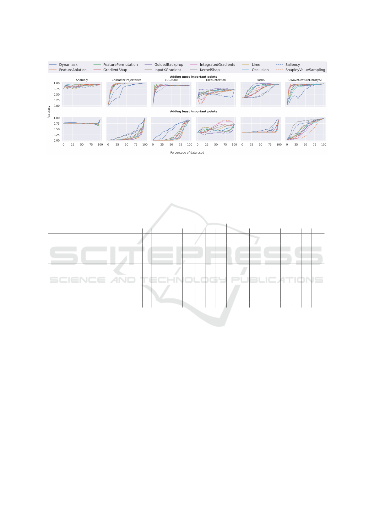
Figure 1: Impact on accuracy. Shows the impact when adding points to the baseline signal using the attribution scores as

sequence order. Top: Shows the increase adding the most important points. Bottom: Shows the increase adding the least

important points. Precisely, each plot read from 100 percent used data to 0 shows the impact removing the least important

points for the top row, respectively the most important for the bottom row. The values show the weighted-f1 scores. Except

Dynamask, Saliency, and KernelShap the performances of the approaches are similar.

Table 4: Prediction agreement. Evaluation of how many data points are required to reach a speciﬁc agreement between the

original and modiﬁed input. All numbers are in percentage, and lower numbers are better as less data was needed to restore

the ground-truth predictions. The numbers in each cell show the percentage of data points added to the baseline to achieve the

required agreement concerning the prediction. Perturbation-based approaches have shown a signiﬁcantly better performance.

Method Anomaly CharacterTraj. ECG5000 FaceDetection FordA UWaveGesture

Req. Agreement in [%] 90 95 100 90 95 100 90 95 100 90 95 100 90 95 100 90 95 100

Gradient-based

GradientShap (Lundberg and Lee, 2017) 1

1 44 97 1

5 18 32 15 20 75 60 71 98 69 77 9

6 1

2 38 100

GuidedBackprop (Springenberg et al., 2014) 1

1 76 98 17 27 45 13 1

4 83 2

2 2

2 5

5 3

3 61 98 1

1 1

6 100

InputXGradient (Shrikumar et al., 2016) 1

1 51 92 16 21 2

9 18 24 4

2 26 36 55 69 81 98 1

2 38 100

IntegratedGradients (Sundararajan et al., 2017) 1

1 3

3 99 1

2 1

5 31 11 18 3

8 63 81 97 70 79 98 1

2 39 100

Saliency (Simonyan et al., 2013) 1

1 76 97 34 41 48 32 37 75 48 51 54 88 93 100 20 53 100

Perturbation-based

Dynamask (Crabb

e and van der Schaar, 2021) 1

1 5 100 55 72 92 18 31 100 100 100 100 50 71 100 61 74 9

FeatureAblation (Zeiler and Fergus, 2014) 1

1 2

2 4

8 1

5 20 2

8 6

6 9

9 60 2

5 3

0 3

5 4

4 5

2 8

2 26 55 9

FeaturePermutation (Fisher et al., 2019)

1 2

2 4

8 1

5 20 2

8 6

6 9

9 60 2

5 3

0 3

5 4

4 5

2 8

2 26 55 9

Occlusion (Zeiler and Fergus, 2014) 1

1 3 83 19 20 2

9 9 15 4

6 1

6 47 87 43 5

5 9

6 33 68 100

Others

KernelShap (Lundberg and Lee, 2017) 1

1 58 100 1

5 22 43 8

8 15 84 70 84 99 90 94 98 16 34 100

Lime (Ribeiro et al., 2016) 1

1 90 100 1

5 1

7 49 8

8 17 75 49 52 81 79 86 99 13 1

7 100

ShapleyValueSampling (Mitchell et al., 2021) 1

1 30 5

1 1

2 1

3 30 10 18 71 68 90 93 65 79 97 9

9 1

5 100

dataset required every method to include almost every

point.

5.3 Inﬁdelity & Sensitivity

The Inﬁdelity measurements provide information

about the change concerning the predictor function

when perturbations to the input are applied. The met-

ric derives from the completeness property of well-

known attribution methods and is used to evaluate

the quality of an attribution method. In the results

in Table 5 the Inﬁdelity represents a mean error us-

ing 100 perturbed samples for each approach. A

lower Inﬁdelity value corresponds to a better attribu-

tion method, and the optimal Inﬁdelity value should

be zero. The results show that the tested methods do

differ by a large margin of less than 7.2% on average,

and in addition, the Inﬁdelity values strongly depend

on the dataset. Neither the gradient-based approaches

nor the perturbation-based or other approaches are su-

perior. The mean increase of the worst-performing

and the best method was 7.2%. The experiments iden-

tiﬁed the highest increases for the CharacterTrajec-

tories dataset (15.8%) and the lowest for the FordA

(3.4%).

Further, the Sensitivity of the methods for a sin-

gle sample was compared. Computationally, the Sen-

sitivity is much more expensive but provides a good

idea about the change in the attribution when the in-

put is perturbed. Using the Sensitivity the robustness

against of the methods concerning noise was evalu-

ated. Ultimately, an attribution method tends to show

low Sensitivity, although this depends on the model

itself. In Table 6 the results of the Sensitivity for all

methods are presented. The results show that Dy-

namask has a Sensitivity of zero. Dynamask by de-

sign forces the importance values to be either one or

zero. Although this is a beneﬁt concerning the Sen-

ICAART 2022 - 14th International Conference on Agents and Artiﬁcial Intelligence

566

Table 5: Inﬁdelity comparison. Computed values show the average Inﬁdelity over the 100 sample subsets. Results show

differences between the different methods when applied to time series data. No category has shown a superior performance,

although the gradient-based approaches were slightly better.

Method Anomaly CharacterTrajectories ECG5000 FaceDetection FordA UWaveGestureLibraryAll

Gradient-based

GradientShap 2.3803 1

8 0

7 0.0014 1.3734 11.4717

GuidedBackprop 2.4057 1.1665 0.8060 0.0014 1.3782 11.6886

InputXGradient 2

6 1

5 0.8135 0.0014 1.3854 11.5830

IntegratedGradients 2.3594 1.2064 0.8260 0

3 1

7 1

Saliency 2.3788 1

1 0.8174 0.0014 1

6 11.7546

Perturbation-based

Dynamask 2.4382 1.2650 0.8271 0

3 1.3806 11.6034

FeatureAblation 2.3859 1.1513 0.8459 0.0014 1.3869 11.5511

FeaturePermutation

2.4015 1.1654 0

9 0.0014 1.3991 11.5112

Occlusion 2

0 1.2078 0.8107 0.0014 1.3752 1

Others

KernelShap 2.4115 1.1802 0.8288 0.0014 1.3785 11.6568

Lime 2.4259 1.1584 0

0 0.0014 1

2 11.6323

ShapleyValueSampling 2

2 1.1671 0.8153 0.0014 1.3745 1

Table 6: Sensitivity comparison. Computed values show the Sensitivity of a sample. Results show larger values for Lime

and Shap-based approaches. Overall the performance of the perturbation-based approaches was superior to most of the other

approaches.

Method Anomaly CharacterTrajectories ECG5000 FaceDetection FordA UWaveGestureLibraryAll

Gradient-based

GradientShap 0.9364 0.6610 0.9149 0.9764 1.0369 1.0347

GuidedBackprop 0.1324 0.1531 0.0562 0.1339 0

8 0.2057

InputXGradient 0.1890 0.1017 0.0709 0.0952 0.0924 0.1927

IntegratedGradients 0.1166 0.1144 0.0458 0

9 0.0906 0.2086

Saliency 0.1902 0.1126 0.1841 0.0995 0.0762 0.2220

Perturbation-based

Dynamask 0

0 0

FeatureAblation 0

4 0

0 0

0 0.0581 0.0463 0

FeaturePermutation 0

4 0

0 0

0 0.0581 0.0463 0

Occlusion 0.0645 0

7 0

5 0

6 0

4 0

Others

KernelShap 1.0908 0.9405 0.2162 0.9248 0.8876 1.0283

Lime 0.8221 0.4986 0.1408 1.5613 0.6974 0.6378

ShapleyValueSampling 0.9132 0.3917 0.1852 0.5938 0.5536 0.3458

sitivity it results in a drawback when ranking the fea-

tures as shown in the accuracy drop experiment. In

addition, perturbation-based approaches have shown

30.9% better results on average concerning their Sen-

sitivity across all datasets. The FordA dataset has

shown the most signiﬁcant difference between the

attribution methods (42.1%), while the Character-

Trajectories dataset has shown the lowest (26.1%).

Besides, the impressive performance of Dynamask,

the Occlusion, FeatureAblation, and FeaturePermuta-

tion have shown results underlining their robustness

against permutations.

5.4 Runtime

The runtime and resource consumption are important

aspects. Even though, the availability of resources

increases, they are not unlimited. Depending on the

throughput of the approach real-time interpretability

can be possible. For mobile devices, the computation

capacity is limited, and low resource dependencies are

beneﬁcial. A Quad-Core Intel Xeon processor, Nvidia

GeForce GTX 1080 Ti, and 64 GB memory were used

to compare the methods concerning their computa-

tional effort. The attribution and execution time for a

single sample of each dataset was computed. In Fig-

ure 2 shows that especially the simple gradient-based

methods like the Saliency, IntegradtedGradients, and

InputXGradient show a low computation time. On the

other side methods like KernelShap and ShapleyVal-

ueSampling have shown increased time consumption.

There is always the trade-off between how many sam-

ples are processed and the computational costs using

SVS and KernelShap. During The analysis, the de-

fault values suggested in the corresponding papers of

the methods were used. In the case of the FaceDetec-

tion dataset, the computational overhead of the Fea-

tureAblation, FeaturePermutation, and Occlusion in-

creased a lot as they strongly depend on the number

of features. The FaceDetection dataset needs 41 times

longer than the anomaly dataset. Overall the compu-

tation time of the FaceDeteciton dataset is four times

longer than the aggregated computation of all others.

The characteristics of the FaceDetection dataset favor

Time to Focus: A Comprehensive Benchmark using Time Series Attribution Methods

567

Figure 2: Time comparison. Shows the time spend to com-

pute the attribution of a single sample. Note that some bars

are not visible due to their fast computation time compared

to the other methods and the time of Dynamask is lowered

by parameter optimization due to the otherwise unsuitable

time consumption. Hardware: Quad-Core Intel Xeon pro-

cessor, Nvidia GeForce GTX 1080 Ti, and 64 GB memory.

methods that are independent of the number of fea-

tures. The high number of channels and time-steps

when every data feature gets evaluated separately in-

creases up to an unacceptable point. In addition, it

has to be mentioned that only 100 epochs instead of

the default 1, 000 for each optimization of Dynamask

were used to lower the computation times. The re-

sults show that this does not change the overall results

of Dynamask but lowers the computational time by a

factor of ten. Using the default 1000 epochs would

not be suitable in any case as the computation time

would increase by a factor of ten.

5.5 Attribution Correlation

Another aspect is the correlation of the different

attribution maps. Therefore, different correlation

measurements were used, namely the Pearson cor-

relation (Benesty et al., 2009), Spearman correla-

tion (Myers and Sirois, 2004) and Jaccard Similar-

ity (Niwattanakul et al., 2013). The Pearson correla-

tion measures the correlation between two series con-

cerning their values. Spearman correlation is a ranked

measurement that compares the ranks for each of the

features. Finally, the Jaccard Similarity is used as a

set-based measurement. During this experiment, the

similarity of the attributions computed over the 100

test sample subsets was evaluated. Ultimately, only

the important points matter concerning a correct attri-

bution. That means intuitively, the similarity of the

methods concerning irrelevant points. To consider

that, percentile subsets of the important features were

selected for the Jaccard Similarity to understand the

agreement of the methods concerning those features.

Summarizing the different similarity and correlation

metrics, the absolute correlation using the Pearson

correlation, the ranking using the Spearman correla-

tion, and the important set of features using the Jac-

card similarity were used.

Figure 3 shows the results. The correlation ma-

trices for the CharacterTrajectories and FordA dataset

(a) CharacterTrajectories

(b) FordA

Figure 3: Attribution correlation Shows the average cor-

relation/similarity of over 100 attributions. The ten percent

most important features were selected for the Jaccard simi-

larity. The method names are shortened using only the cap-

ital characters. KernelShap shows a signiﬁcantly lower cor-

relation to other methods compared to all others. Feature

Ablation and FeaturePermutation have shown a high corre-

lation.

as the other datasets have similar show results. Over-

all every matrix shows the same behavior. Feature-

Ablation (FA) and FeaturePermutation (FP) are very

similar. In addition, the Dynamask (D) approach and

KernelShap (KS) are different from any of the others.

This difference is the case for Dynamask, as the tech-

nique only makes a binary decision if a feature is sig-

niﬁcant or not. Intuitively, this should result in a high

similarity for the Jaccard measurement. However, this

is not the case as the attribution of Dynamask has an

internal smoothing based on the loss used to optimize

the mask. This smoothing will include less important

features in the important feature set to preserve a con-

tinuous mask. Furthermore, Lime (L) and KernelShap

(KS) seemed less similar to the other approaches.

5.6 Dependency on Model Parameter

Attribution methods should depend on the model

parameter and the labels of the data. Therefore,

the impact of label permutation and parameter ran-

domization of the model was evaluated. The paper

only shows the results using the CharacterTrajectories

dataset as the results on the other datasets are similar.

The idea of the label permutation is that attribu-

tion methods should depend heavily on the labels.

Good results in this experiment show a high intrin-

ICAART 2022 - 14th International Conference on Agents and Artiﬁcial Intelligence

568

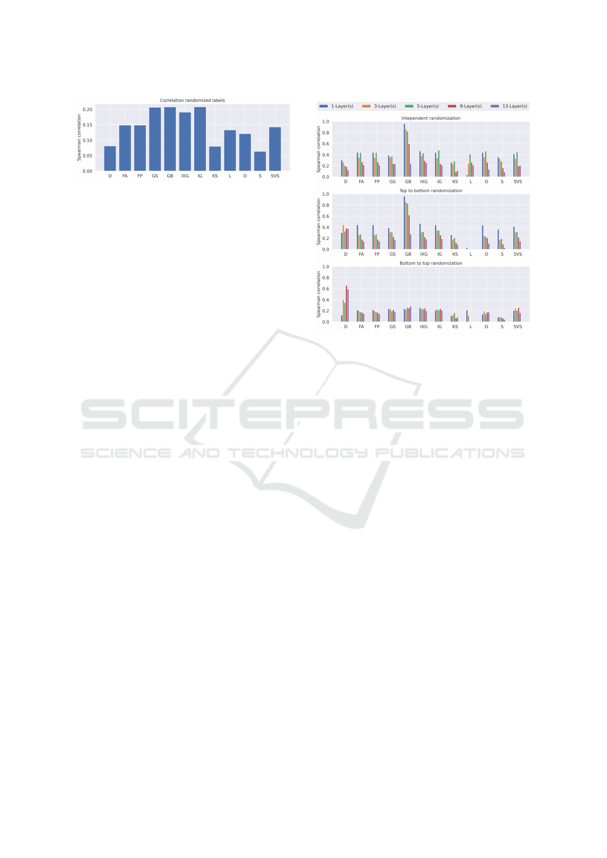
Figure 4: Attribution comparison. Shows the Spearman

correlation (rank correlation) of the attribution methods

evaluated on the same model architecture using randomized

training labels using the CharacterTrajectories dataset. The

method names are shortened using only the capital charac-

ters. Dynamask, KernelShap, and Saliency show a signiﬁ-

cantly lower dataset dependence.

sic data characteristic dependence which is not a de-

sired feature of an attribution method. The models

were trained similar to the baseline model on the same

training data but permuted the labels. This permuta-

tion results in a model that does not generalize well

but learns to replicate the training set. In addition,

this approach did not require the validation dataset.

The accuracies of those models are very high for the

training set. Nevertheless, they fail on the test set.

Precisely speaking, these models do not have a label

dependence. All models reached a near-perfect per-

formance on the training set. Figure 4 highlights that

the correlation drops down to values between 0.05 and

0.2. Based on the overall low correlation, the attribu-

tion methods highly depend on the labels rather than

dataset characteristics. GradientShap, GuidedBack-

prop, InputXGradient, and IntegratedGradients have

shown three times larger correlations in contrast to

Dynamak, KernelShap, and Saliency. However, their

correlation is still low enough to justify the label de-

pendency.

In addition to the label permutation, layers of a

correctly trained network were systematically ran-

domized to understand the dependency concerning

the model parameters. To understand the impact of

the layers, each layer was randomized independently.

Further, the model was randomized starting from the

bottom to the top and vice-versa. The results in Fig-

ure 5 show all three approaches. Interestingly, the

correlation of GuidedBackprop stays high when ran-

domizing the top layers but signiﬁcantly drops when

randomizing the bottom layers. Randomizing the up-

per layers, the correlation of Guidedbackprop is close

to the original attribution map, whereas the correla-

tion of the other methods drops by 0.5 or more. That

suggests that this method is more based on the values

of the ﬁrst few layers. In addition, the results show

that for all attribution techniques, a single random-

ized layer is enough to get an attribution that is no

longer related to the original attribution map. This

Figure 5: Correlation to original attribution. Shows the

Spearman correlation of the attribution methods evaluated

on the trained model and randomized layer weights using

the CharacterTrajectories dataset. Weights are either ran-

domized for each layer independently, from top to the bot-

tom layer or vice versa. Only layers with trainable param-

eters (conv, batchnorm, dense) are included when counting

the number of randomized layers. The method names are

shortened using only the capital characters. GuidedBack-

prop shows signiﬁcant correlations when only the upper

layers are randomized. The correlation of all other meth-

ods drops signiﬁcantly.

high dependency on the model parameter is the de-

sired property. The top to bottom randomization fur-

ther shows that except for the Dynamsk approach, the

correlation continuously gets smaller when random-

izing more layers. Finally, the bottom to top random-

ization highlights that the randomization of the ﬁrst

layer of the network is enough to produce attribution

maps that are not related to the original.

5.7 Visual Attribution Comparison

Figure 6 shows all computed attribution maps for a

reference sample. Due to interpretability reasons, an

anomalous instance of the anomaly dataset was se-

lected. The example in the top left corner contains a

single anomaly in one channel that is important for

the classiﬁcation. The rest of the ﬁgure shows the

different attribution maps and the impact of random-

ization on the methods. The ﬁgure shows the robust-

ness to randomized parameters. In the second col-

umn, the Integrated gradients approach was able to

ﬁnd the peak. This column corresponds to a model

trained on randomized labels. Therefore, the model

Time to Focus: A Comprehensive Benchmark using Time Series Attribution Methods

569

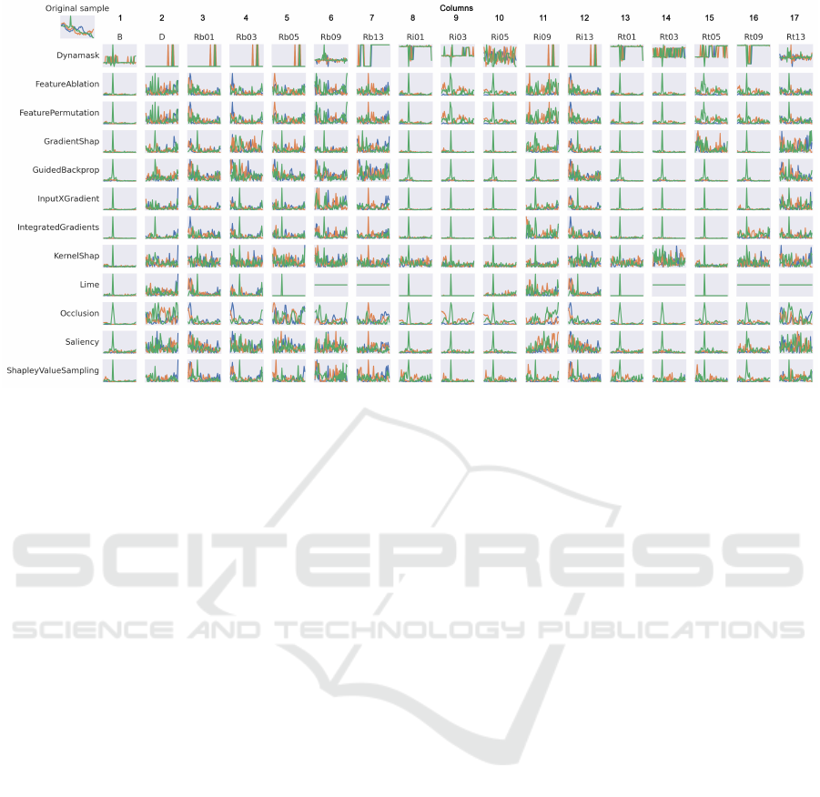
Figure 6: Visual comparison. Shows all attributions for a selected anomaly sample. The important part is the peak of the

sample. ’Ri’, ’Rb’, ’Rt’, ’D’, and ’B’ correspond to the independent, bottom to top, top to bottom randomization, label

randomization, and original attribution map. Only conv, batchnorm, and dense layers are counted. Changing the data labels

during training signiﬁcantly worsens the performance of all approaches except IntegratedGradients for the anomaly dataset.

Overall randomizing lower layers resulted in much more noise compared to randomization in the upper layers.

used in column two is not generalized and learned

only to map the training data. Columns three to seven

show a model randomization starting from the bottom

layers. The results show that some methods still per-

form well when only one or three layers starting from

the bottom are randomized other attribution methods

directly collapsed. Columns eight to twelve show

the independent layer randomization. Except for Dy-

namask, the attribution techniques were able to deal

with up to handle the layer randomization in the up-

per layer of the network quite well, whereas all attri-

bution methods collapsed when the lower layers were

randomized. Columns thirteen to seventeen show the

randomization starting from the top of the network.

Most attribution methods were able to recover from

the randomization for a high number of randomized

layers. Overall the randomization of the lower lay-

ers changed the attribution much more concerning the

noise. Interestingly, changes in the upper layers did

not affect the attribution methods that much.

5.8 Continuity

One aspect that is missing most times is attribution

continuity. In the image domain, the use of superpix-

els solves this problem. However, in the time series

domain, it is not that easy. Most of the attribution

methods do not consider groups of values. In Table 7

shows the evaluation of the continuity. The continuity

calculates the absolute difference between the attribu-

tion value of a point t and t + 1 for each time-step and

each channel. Using the mean across a sample pro-

vides a value that indicates how continuous the ex-

planation is. Lower values correspond to an explana-

tion that does not contain many switches from impor-

tant to not important features. This measurement was

computed over the 100 attributed samples and took

the mean for each dataset. The results indicate that

the perturbation-based approaches favor continuous

explanations. Gradient-based methods overall have

shown the worst performance. One reason for this

is the noisy gradients used to compute the attribution

maps.

6 DISCUSSION

A summarization and discussion in a detailed man-

ner is offered to provide on choosing an attribution

method. The different aspects and application scenar-

ios are described below. First, it has to be mentioned

that every attribution method has shown satisfying re-

sults. However, the choice of an attribution method

should depend on the required characteristics. The

overall results are presented in Table 8. Teh resuls

highlight that choosing an attribution method can be

very important, as mentioned by Vermeire et al. (Ver-

meire et al., 2021).

Starting with the accuracy drop, the evaluation

shows to which extend the methods rank the most

ICAART 2022 - 14th International Conference on Agents and Artiﬁcial Intelligence

570

Table 7: Continuity comparison. Computed values show the mean continuity of the attribution maps. Lower values cor-

respond to continuous maps. Continuity was calculated by shifting the attribution map, subtracting if from the original one,

taking the absolute values, and computing the mean. Lower values are better. Perturbation-based methods have been shown to

outperform gradient-based with respect to the continuity on almost all datasets. Speciﬁcally, Dynamask and Occlusion have

been shown to perform well across all datasets.

Method Anomaly CharacterTrajectories ECG5000 FaceDetection FordA UWaveGestureLibraryAll

Gradient-based

GradientShap 0.0947 0.0368 0.0616 0.0613 0.0813 0.0543

GuidedBackprop 0.1201 0.0537 0.0913 0.0957 0

1 0

InputXGradient 0.0801 0.0390 0.0508 0.0620 0.0855 0.0537

IntegratedGradients 0.0864 0.0369 0.0609 0.0632 0.0858 0.0508

Saliency 0.1176 0.0748 0.1439 0.1170 0.1229 0.0842

Perturbation-based

Dynamask 0

2 0

4 0

2 0

7 0

9 0

FeatureAblation 0.0784 0.0395 0.0584 0.0624 0.0815 0.0601

FeaturePermutation 0.0784 0.0395 0.0584 0.0624 0.0815 0.0601

Occlusion 0

3 0

9 0

7 0

5 0

Others

KernelShap 0.1423 0.1086 0.0641 0.1671 0.1973 0.1795

Lime 0.1122 0.0496 0

8 0

0 0.0883 0.0928

ShapleyValueSampling 0

3 0

5 0.0505 0.0583 0.0885 0.0713

Table 8: Overall Evaluation. Overall results with respect

to the different aspects evaluated in this paper. A = Accu-

racy Impact / Agreement, I = Inﬁdelity, S = Sensitivity, R =

Runtime, Ld = Label dependency, Md = Model Parameter

Dependency, C = Continuity.

Method A I S R Ld Md C

Gradient-based

GradientShap ⊕ ⊕

GuidedBackprop ⊕ ⊕ 

InputXGradient ⊕ ⊕

IntegratedGradients ⊕ ⊕

Saliency  ⊕ ⊕ ⊕

Perturbation-based

Dynamask  ⊕  ⊕ ⊕

FeatureAblation ⊕ ⊕ 

FeaturePermutation ⊕ ⊕ 

Occlusion ⊕ ⊕  ⊕

Others

KernelShap   ⊕

Lime ⊕ ⊕ ⊕ ⊕

ShapleyValueSampling ⊕  ⊕

and least signiﬁcant features based on the impact on

the accuracy. Most of the methods were able to

show high-quality results across all datasets. How-

ever, there were some outstanding performances.

Speciﬁcally, the perturbation-based were able to per-

form slightly better than the other methods on some

datasets. Saliency and Dynamask have shown some

weaknesses for some datasets, such as the Character-

Trajectories and FordA. Both methods require further

adjustments and knowledge about the data to achieve

good results. One example is the ratio of signiﬁcant

points for the Dynamask approach to select the cor-

rect number of features. If additional information is

available, such as the ratio of selected features, meth-

ods like Dynamask can express their full potential.

The attribution agreement shows similar results.

Concerning Inﬁdelity and Sensitivity, every

method performed well, and no approach suffered

more. The results show that gradient-based meth-

ods obtained the best Inﬁdelity results. It was

the opposite for the Sensitivity. Especially, Gradi-

entShap, InputXGradient, and Saliency approaches

are robust against signiﬁcant perturbations in the in-

put space (Inﬁdelity). On the other side, the Dyna-

mask, FeaturePermutation, and Occlusion approaches

have shown good robustness concerning changes in

the attribution when small perturbations to the input

are applied (Sensitivity). Dynamask has a loss that

forces a binary decision whether a feature is selected

or not ensures this behavior. Using attribution meth-

ods with low Sensitivity values in cases where adver-

sarial attacks can occur is suggested.

The runtime aspect gets critical when the use case

requires near real-time explanations. In addition, the

results have shown that the dataset characteristics are

relevant. The ﬁndings show that approaches based on

the sequence length and number of channels suffer

from very high runtimes for single samples. These

runtimes make it impossible to use them in a real-

time scenario. However, if the time consumption is

not of interest, this aspect is not relevant. Further-

more, gradient-based methods are less dependent on

the dataset characteristics and very suitable when time

matters. Contrarily, besides Dynamask and Lime, the

perturbation-based approaches suffer from the num-

ber of features. In the case of Lime, the number of

samples required to populate the space to train the

surrogate model increases with a higher number of

features. Dynamask does not suffer from the feature

number. However, the approach needs an additional

training phase. This training requires multiple epochs

Time to Focus: A Comprehensive Benchmark using Time Series Attribution Methods

571

and in addition repetitions based on the different ar-

eas checked during the training. Ultimately, the back-

propagation needs resources and time. Based on the

computational times, the use of ShapelyValueSam-

pling and KernelShap in real-time scenarios is nearly

impossible. For completeness, it has to be mentioned

that it is possible to tweak hyperparameters.

The label permutation and layer randomization

provided insights concerning the role of the model

parameters during the attribution computation. Intu-

itively, all methods have shown a high dependency

on the labels of the data. Training a model with ran-

domized targets has shown, the attributions depend on

the labels as they should. Although all methods have

shown this dependency, the Saliency, Dynamask, Ker-

nelShap, and Lime have shown more dependence on

the targets. Concerning the model parameters, the

results show that randomizing any layer results in

changes of the attribution maps. Besides, the Guided-

Backprop attribution maps signiﬁcantly change after

any modiﬁcation. Speciﬁcally, Lime collapses com-

pletely. This collapse emphasizes that Lime directly

depends on the model, and GuidedBackprop is rely-

ing more on data. An explanation for this behavior is

that some methods detect dataset differences. Espe-

cially in the image domain, it was shown that some

attribution methods can act like an edge detectors.

Finally, continuity plays a pivotal role in human

understanding. In use cases that include human eval-

uation, it is beneﬁcial to have continuous attribu-

tion maps. Imagine there is a signiﬁcant frame with

many important but some less important features. It

might be superior to mark the whole window as im-

portant, although this covers some insigniﬁcant fea-

tures. In the time series domain, the context mat-

ters, and continuous attribution maps are easier to un-

derstand. The results show that the Dynamask ap-

proach, Lime, Occlusion, and ShapleyValueSampling

are superior concerning their continuity. Intuitively,

the attribution maps produced by gradient-based tech-

niques look noisy, whereas permutation-based look

smoother. Dynamask includes a loss term that ensures

a smoother attribution map. Lime and ShapleyValue-

Sampling produce smoother maps. The results sug-

gest using a perturbation-based approach if a human

inspection is relevant.

Comparing the gradient-based, perturbation-

based, and other approaches, every category has

shown advantages over the other category in some

aspects. Generally, gradient-based methods are fast,

show high Inﬁdelity, label dependency but are noisy,

not continuous, and suffer concerning the Sensitivity.

In contrast to gradient-based methods, perturbation-

based approaches produce continuous maps, shine

concerning the Sensitivity, label dependency but suf-

fer when it comes to the runtime.

7 CONCLUSION

A comprehensive evaluation of a large set of state-of-

the-art attribution methods applicable to time series

was performed. The results show that most attribu-

tion methods can identify signiﬁcant features with-

out prior knowledge about the data. In the evalua-

tion, the perturbation-based approaches have shown

slightly superior performance in the data occlusion

game. In addition, the results are validated by mea-

suring the agreement of the methods using differ-

ent correlation and similarity measurements. Except

for Dynamask and KernelShap, the correlation be-

tween the attribution methods showed high values.

Further experiments were conducted to highlight the

high dependence of the attribution methods on the

model and the target labels. Only Guided-Backprop

has shown lower reliance on the top layers of the

network. Concerning Inﬁdelity, the gradient-based

attribution methods showed superior performance.

The perturbation-based attribution methods are su-

perb concerning Sensitivity and continuity. Continu-

ity is an important aspect when it comes to human

interpretability. The results hold across a set of dif-

ferent tasks, sequence lengths, feature channels, and

the number of samples. Furthermore, the results show

that the choice of an attribution method depends on

the target scenario, and different aspects like runtime,

accuracy, continuity, noise are indispensable.

ACKNOWLEDGMENT

This work was supported by the BMBF projects Sen-

sAI (BMBF Grant 01IW20007) and the ExplAINN

(BMBF Grant 01IS19074). We thank all members of

the Deep Learning Competence Center at the DFKI

for their comments and support.

REFERENCES

Abdul, A., von der Weth, C., Kankanhalli, M., and Lim,

B. Y. (2020). Cogam: Measuring and moderating cog-

nitive load in machine learning model explanations. In

Proceedings of the 2020 CHI Conference on Human

Factors in Computing Systems, pages 1–14.

Adebayo, J., Gilmer, J., Muelly, M., Goodfellow, I., Hardt,

M., and Kim, B. (2018). Sanity checks for saliency

maps. arXiv preprint arXiv:1810.03292.

ICAART 2022 - 14th International Conference on Agents and Artiﬁcial Intelligence

572

Allam, Z. and Dhunny, Z. A. (2019). On big data, artiﬁcial

intelligence and smart cities. Cities, 89:80–91.

Ancona, M., Ceolini, E.,

Oztireli, C., and Gross, M. (2017).

Towards better understanding of gradient-based at-

tribution methods for deep neural networks. arXiv

preprint arXiv:1711.06104.

Ancona, M., Ceolini, E.,

Oztireli, C., and Gross, M. (2019).

Gradient-based attribution methods. In Explainable

AI: Interpreting, Explaining and Visualizing Deep

Learning, pages 169–191. Springer.

Bagnall, A., Lines, J., Vickers, W., and Keogh, E. (2021).

The uea & ucr time series classiﬁcation repository.

Benesty, J., Chen, J., Huang, Y., and Cohen, I. (2009).

Pearson correlation coefﬁcient. In Noise reduction in

speech processing, pages 1–4. Springer.

Bibal, A., Lognoul, M., de Streel, A., and Fr

enay, B. (2020).

Impact of legal requirements on explainability in ma-

chine learning. arXiv preprint arXiv:2007.05479.

Crabb

e, J. and van der Schaar, M. (2021). Explaining time

series predictions with dynamic masks. In Proceed-

ings of the 38-th International Conference on Machine

Learning (ICML 2021). PMLR.

Das, A. and Rad, P. (2020). Opportunities and challenges

in explainable artiﬁcial intelligence (xai): A survey.

arXiv preprint arXiv:2006.11371.

silovi

c, F. K., Br

c, M., and Hlupi

c, N. (2018). Ex-

plainable artiﬁcial intelligence: A survey. In 2018 41st

International convention on information and commu-

nication technology, electronics and microelectronics

(MIPRO), pages 0210–0215. IEEE.

Fisher, A., Rudin, C., and Dominici, F. (2019). All mod-

els are wrong, but many are useful: Learning a vari-

able’s importance by studying an entire class of pre-

diction models simultaneously. J. Mach. Learn. Res.,

20(177):1–81.

Huber, T., Limmer, B., and Andr

e, E. (2021). Benchmark-

ing perturbation-based saliency maps for explaining

deep reinforcement learning agents. arXiv preprint

arXiv:2101.07312.

Ivanovs, M., Kadikis, R., and Ozols, K. (2021).

Perturbation-based methods for explaining deep neu-

ral networks: A survey. Pattern Recognition Letters.

Karliuk, M. (2018). Ethical and legal issues in artiﬁcial

intelligence. International and Social Impacts of Arti-

ﬁcial Intelligence Technologies, Working Paper, (44).

Lundberg, S. M. and Lee, S.-I. (2017). A uniﬁed approach

to interpreting model predictions. In Proceedings of

the 31st international conference on neural informa-

tion processing systems, pages 4768–4777.

Mitchell, R., Cooper, J., Frank, E., and Holmes, G. (2021).

Sampling permutations for shapley value estimation.

arXiv preprint arXiv:2104.12199.

Myers, L. and Sirois, M. J. (2004). Spearman correla-

tion coefﬁcients, differences between. Encyclopedia

of statistical sciences, 12.

Nielsen, I. E., Rasool, G., Dera, D., Bouaynaya, N.,

and Ramachandran, R. P. (2021). Robust ex-

plainability: A tutorial on gradient-based attribution

methods for deep neural networks. arXiv preprint

arXiv:2107.11400.

Niwattanakul, S., Singthongchai, J., Naenudorn, E., and

Wanapu, S. (2013). Using of jaccard coefﬁcient for

keywords similarity. In Proceedings of the interna-

tional multiconference of engineers and computer sci-

entists, volume 1, pages 380–384.

Perc, M., Ozer, M., and Hojnik, J. (2019). Social and juristic

challenges of artiﬁcial intelligence. Palgrave Commu-

nications, 5(1):1–7.

Peres, R. S., Jia, X., Lee, J., Sun, K., Colombo, A. W.,

and Barata, J. (2020). Industrial artiﬁcial intelligence

in industry 4.0-systematic review, challenges and out-

look. IEEE Access, 8:220121–220139.

Ribeiro, M. T., Singh, S., and Guestrin, C. (2016). ”why

should I trust you?”: Explaining the predictions of any

classiﬁer. In Proceedings of the 22nd ACM SIGKDD

International Conference on Knowledge Discovery

and Data Mining, San Francisco, CA, USA, August

13-17, 2016, pages 1135–1144.

Shrikumar, A., Greenside, P., Shcherbina, A., and Kun-

daje, A. (2016). Not just a black box: Learning im-

portant features through propagating activation differ-

ences. arXiv preprint arXiv:1605.01713.

Siddiqui, S. A., Mercier, D., Munir, M., Dengel, A., and

Ahmed, S. (2019). Tsviz: Demystiﬁcation of deep

learning models for time-series analysis. IEEE Ac-

cess, 7:67027–67040.

Simonyan, K., Vedaldi, A., and Zisserman, A. (2013).

Deep inside convolutional networks: Visualising im-

age classiﬁcation models and saliency maps. arXiv

preprint arXiv:1312.6034.

Springenberg, J. T., Dosovitskiy, A., Brox, T., and Ried-

miller, M. (2014). Striving for simplicity: The all con-

volutional net. arXiv preprint arXiv:1412.6806.

Sundararajan, M., Taly, A., and Yan, Q. (2017). Axiomatic

attribution for deep networks. In International Confer-

ence on Machine Learning, pages 3319–3328. PMLR.

Vermeire, T., Laugel, T., Renard, X., Martens, D., and De-

tyniecki, M. (2021). How to choose an explainability

method? towards a methodical implementation of xai

in practice. arXiv preprint arXiv:2107.04427.

Yeh, C.-K., Hsieh, C.-Y., Suggala, A., Inouye, D. I., and

Ravikumar, P. K. (2019). On the (in) ﬁdelity and sen-

sitivity of explanations. Advances in Neural Informa-

tion Processing Systems, 32:10967–10978.

Zeiler, M. D. and Fergus, R. (2014). Visualizing and under-

standing convolutional networks. In European confer-

ence on computer vision, pages 818–833. Springer.

Zhang, Q. and Zhu, S.-C. (2018). Visual interpretabil-

ity for deep learning: a survey. arXiv preprint

arXiv:1802.00614.

Time to Focus: A Comprehensive Benchmark using Time Series Attribution Methods

573