A Machine Learning Approach for Spare Parts Lifetime Estimation
Lu
´
ısa Macedo
1
, Lu
´
ıs Miguel Matos
1 a
, Paulo Cortez
1 b
, Andr
´
e Domingues
1
, Guilherme Moreira
2
and Andr
´
e Pilastri
3 c
1
ALGORITMI Center, Dep. Information Systems, University of Minho, Guimar
˜
aes, Portugal
2
Bosch Car Multimedia, Braga, Portugal
3
EPMQ - IT Engineering Maturity and Quality Lab, CCG ZGDV Institute, Guimar
˜
aes, Portugal
Keywords:
Explainable Artificial Intelligence, Maintenance Data, Regression, Remaining Useful Life (RUL).
Abstract:
Under the Industry 4.0 concept, there is increased usage of data-driven analytics to enhance the production
process. In particular, equipment maintenance is a key industrial area that can benefit from using Machine
Learning (ML) models. In this paper, we propose a novel Remaining Useful Life (RUL) ML-based spare part
prediction that considers maintenance historical records, which are commonly available in several industries
and thus more easy to collect when compared with specific equipment measurement data. As a case study, we
consider 18,355 RUL records from an automotive multimedia assembly company, where each RUL value is
defined as the full amount of units produced within two consecutive corrective maintenance actions. Under
regression modeling, two categorical input transforms and eight ML algorithms were explored by consid-
ering a realistic rolling window evaluation. The best prediction model, which adopts an Inverse Document
Frequency (IDF) data transformation and the Random Forest (RF) algorithm, produced high-quality RUL pre-
diction results under a reasonable computational effort. Moreover, we have executed an eXplainable Artificial
Intelligence (XAI) approach, based on the SHapley Additive exPlanations (SHAP) method, over the selected
RF model, showing its potential value to extract useful explanatory knowledge for the maintenance domain.
1 INTRODUCTION
Maintenance is a key area within the Industry 4.0
concept. Indeed, equipment maintenance can have
a significant impact on the uptime and efficiency of
the entire production system (Lee et al., 2019). It is
estimated that between 15% and 40% of total pro-
duction costs are attributed to maintenance. Thus,
a good maintenance policy is essential to ensure the
efficiency of the industrial system and increase the
reliability of equipment (Wang, 2012). Following
the fourth industrial revolution, there is an increase
in data availability, which leads to opportunities for
changing the maintenance paradigm (Susto et al.,
2012). The integration between the physical and dig-
ital systems of production environments allows more
significant volumes of data collection, from different
equipments and sections of the plant, enabling a faster
exchange of information (Rauch et al., 2020; Borgi
a
https://orcid.org/0000-0001-5827-9129
b
https://orcid.org/0000-0002-7991-2090
c
https://orcid.org/0000-0002-4380-3220
et al., 2017). Through analytical approaches, the col-
lected data can potentially provide valuable insights
into the industrial process, improving decision mak-
ing, which can result in a reduction of maintenance
costs and machine failures and an increase of the use-
ful life of spare parts (Carvalho et al., 2019).
Several maintenance approaches and strategies
have emerged, which can be grouped into three main
categories (Susto et al., 2012; Susto et al., 2015):
• Run-to-Failure (R2F) or Corrective Maintenance
which occurs whenever a piece of equipment
stops working. It is the simplest maintenance
strategy since it is executed as soon as an equip-
ment failure is detected. This approach con-
tributes to higher maintenance costs, given the im-
mediate requirement of labor and parts to repair.
• Preventive Maintenance (PvM), Time-based
Maintenance or Scheduled Maintenance, is a type
of maintenance that is performed periodically,
with a planned schedule, in order to anticipate
equipment failures.
Macedo, L., Miguel Matos, L., Cortez, P., Domingues, A., Moreira, G. and Pilastri, A.
A Machine Learning Approach for Spare Parts Lifetime Estimation.
DOI: 10.5220/0010903800003116
In Proceedings of the 14th International Conference on Agents and Artificial Intelligence (ICAART 2022) - Volume 3, pages 765-772
ISBN: 978-989-758-547-0; ISSN: 2184-433X
Copyright
c
 2022 by SCITEPRESS – Science and Technology Publications, Lda. All rights reserved
765

• Predictive Maintenance (PdM) is a more recent
type of maintenance, which emerged with the
modernization of industrial processes and integra-
tion of sensors in equipment/production lines. It
uses predictive tools (data-driven) to continuously
monitor a piece of equipment or process, evaluat-
ing and calculating when maintenance is required.
It also allows an early detection of failures by typ-
ically implementing Machine Learning (ML) al-
gorithms based on historical equipment data.
Most industries opt for a hybrid system that in-
cludes a corrective (R2F) and preventive (PvM) main-
tenance, where the former strategy being executed
when a failure is detected and there is no preventive
maintenance scheduling. However, these two types of
strategies raise have drawbacks. Industries that adopt
a R2F maintenance often delay maintenance actions,
assuming the risk of unavailability of their assets. As
for the PvM maintenance, it might lead to the replace-
ment of spare parts that are far from reaching their
end of life (Carvalho et al., 2019). An alternative is to
adopt a predictive maintenance (PdM), which can po-
tentially detect a failure before it occurs. Yet, PdM is
not a viable option for many industries, since it often
requires the implementation of the particular informa-
tion systems infrastructure, expertise, and customized
intelligent software (Jardine et al., 2006).
Within this context, the Remaining Useful Life
(RUL) emerges as valuable indicator, typically cou-
pled with predictive maintenance systems, to predict
equipment failures. More precisely, RUL estimates
the total time (e.g., in days, months or years) that a
component is capable of performing its function be-
fore justifying its replacement, implying an economic
aspect dependent on the context and its operational
characteristics (Kang et al., 2021; Okoh et al., 2014).
There are two main approaches for RUL predic-
tion: model-based and data-driven methods (Wang
et al., 2020). The model-based relies on statistical es-
timation techniques to model the degradation process
of machines and predict the RUL. On the other hand,
data-driven approaches are more accurate since it uses
sensor data directly from the equipments and then
ML to learn its degradation process, instead of rely-
ing on theoretical knowledge about the failure pro-
cess.(Wang et al., 2020; Li et al., 2020).
RUL equipment/component data-driven predic-
tion remains a key challenge in predictive mainte-
nance, since it requires a data set that covers the entire
period from machine operation to failure, which is rel-
atively difficult to acquire and, due to business issues,
companies are often reluctant to open their data to the
public (Fan et al., 2015). Indeed, most data-driven
RUL prediction studies work with private industry
data, under different ML algorithm approaches. For
instance, (Wu et al., 2017) developed a Random For-
est based prognostic methods to predict the tool wear
in milling operations. More recently, (Cheng et al.,
2020) proposed a data-driven framework for bearing
RUL prediction that uses a Deep Convolution Neu-
ral Network (CNN) to discover a pattern between the
calculated indicator and the bearing vibration signals.
Using the predicted degradation energy indicator, a
Support Vector Regressor was implemented to predict
the RUL of the testing bearings.
Most of the data-driven RUL studies use equip-
ment measurements (e.g., image, temperature levels,
equipment functioning time) as the inputs of a ML
RUL prediction model (Kang et al., 2021; Okoh et al.,
2014). In this paper, we propose a rather different
RUL ML prediction approach, in which the lifetime
of spare parts is predicted based on corrective main-
tenance historical records (which are more easy to
collect). In particular, we measure the lifetime in
terms of the full amount of units produced within
two consecutive corrective maintenance actions. As
a case study, we consider a recent dataset that in-
cludes 18,355 records with RUL measurements that
were extracted from an automotive multimedia as-
sembly company. Assuming a regression task mod-
eling, we explore and compare eight distinct ML al-
gorithms, namely Decision Tree (DT), Random For-
est (RF), Extra Trees (ET), XGBoost (XB), Light
Gradient Boost Machine (LGBM), Histogram-based
Gradient Regression Tree (HGBM), a Gaussian ker-
nel Support Vector Machine (SVM) and Linear Sup-
port Vector Machine (LSVM). Two categorical pre-
processing techniques were employed to handle in-
puts with a high cardinality of distinct levels: Per-
centage Categorical Pruned (PCP) and Inverse Docu-
ment Frequency (IDF). Moreover, the performance of
the ML predictive models was evaluated by assuming
a realistic Rolling Window scheme, which simulates
several training and testing executions through time.
Finally, the best RUL prediction model is further ana-
lyzed in terms of its extracted knowledge by adopting
an eXplainable Artificial Intelligence (XAI) approach
(Sahakyan et al., 2021), namely by using SHapley
Additive exPlanations (SHAP) (Lundberg and Lee,
2017b), which allows to measure the impact of the
adopted industrial inputs in the RUL predictions.
The paper is structured as follows. Section 2 de-
scribes the industrial maintenance data, the proposed
Machine Learning (ML) approaches and the evalua-
tion methodology. Then, Section 3 presents the ob-
tained results. Lastly, the main conclusions are dis-
cussed in Section 4.
ICAART 2022 - 14th International Conference on Agents and Artificial Intelligence
766

2 MATERIALS AND METHODS
2.1 Industrial Data
For this task, 118,776 records of maintenance orders
were collected alongside spare parts movements per-
formed at a major automotive multimedia assembly
company between April 2004 and May 2021. The
data consists of a compilation of maintenance orders
for spare parts replacement within the equipment.
Furthermore, it was possible to register the type of
maintenance for each equipment machine, the techni-
cian who performed it, and the part replaced. The ex-
act order can also be associated with several records,
depending on the variety of parts used for the main-
tenance (e.g., maintenance that requires three differ-
ent spare parts will be represented by three records,
one for each part). The order can also be reopened
whenever there is a new movement of the part. More-
over, there are six distinct types of movements associ-
ated with spare parts: stock entries in maze-supplier,
returns of the parts to the supplier, stock out for a
maintenance order, and return of the part from main-
tenance to maze. There are three types of mainte-
nance orders: corrective, preventive and improvement
(changes performed on the equipment to introduce
improvements).
The data initially supplied did not present any in-
dication regarding the duration of the part, so a strat-
egy of comparing similar records, ordered in time,
was adopted to estimate the total production for which
a part, for a given equipment, can be subject to before
failure. For research purposes, only the movements
performed between the maze-maintenance were ac-
counted for, focusing on the records that present out-
puts of parts for maintenance. The returns of ma-
terial to the warehouse, on the part of maintenance,
were used to make adjustments in the registers, since
there were maintenance orders that ended up not re-
placing parts, and therefore returned in their entirety
to the warehouse. Furthermore, an adjustment was
made on the dataset to account only for the spare parts
whose maintenance was a part replacement, meaning
that there is no record of that specific part to return
to the warehouse. In addition, we collected a new
dataset, containing 4,488,689 daily records, of the
number of parts each piece of equipment produced
between 00:00h and 23:59h on a day. By comparing
the dates of the two maintenance records for the same
equipment, with the same spare part, it was possible
to associate a quantity produced to that transaction,
through the sum of the quantities produced between
the period being compared. The following function
presents the reasoning followed to calculate the target
variable (y):
f (x) ∩ g(x) = f (x +1)∩g(x + 1) =⇒ y =
t(x+1)
∑
i=t(x)
Q(i),
(1)
where f denotes the equipment, g the spare part, t
the date when the transaction was held, Q represents
the production volume and y the spare part lifetime,
in production units. A special attention was paid to
specific maintenance orders for each record to ensure
accuracy in the target calculation. Since the purpose
is to estimate the total lifetime of a part, when com-
paring two transactions, if the second one corresponds
to a preventive maintenance order, the assigned value
is 0, and therefore removed from the dataset. As
mentioned in Section 1, the preventive maintenance
is scheduled, occurring within a specified time limit,
regardless of whether or not there is a need for part
replacement. Thus, we intended to capture the life
of a machine part from the moment it is replaced
within the equipment until it fails, thus being labeled
as ”corrective maintenance”. Therefore, we only cal-
culated the lifetime whenever the second transaction
compared was corrective.
The final dataset contains 18,355 records, over
seven distinct features. As shown in Table 1, all at-
tributes are categorical, with the exception of part life.
There are 1,189 unique types of equipment, in 73 sub-
types, 37 types and three sections, and 3,418 unique
spare parts, from 8 different suppliers, one of them
being the category ”Not Available” which represents
94.6% of the data. The useful life of the spare part
varies from 1 to 17,909,367, having an average value
of 506,026.
Table 1: Adopted data attributes (input features).
Context Attribute Description
spare part
id spare part id: 3418 categorical levels
supplier supplier code: 8 categorical levels
technician technician name : 1709 categorical levels
lifetime spare part lifetime: 12020 levels
equipment
id equipment name: 1189 categorical levels
type equipment type: 37 categorical levels
subtype equipment subtype: 73 categorical levels
section equipment section: 3 categorical levels
2.2 Data Preprocessing
The data preprocessing involved the transformation of
categorical values into numerical values. We com-
pared two transformations that were specifically de-
signed to handle large cardinally categorical inputs
(which is our case): IDF (Matos et al., 2018) and PCP
(Matos et al., 2019). The former transform converts
A Machine Learning Approach for Spare Parts Lifetime Estimation
767

each input into a single numeric value, using a map-
ping that puts the most frequent levels closer to zero
are more distant to each other, while the less frequent
levels appear on the right side of the scale (larger val-
ues) and closer to each other. The latter transform
merges all infrequent levels (10%) into a single “Oth-
ers” level and then employs the popular one-hot en-
coding that uses one boolean value per level. All tech-
niques were implemented through the Python library
Cane (Matos et al., 2020). The categorical encodings
were calculated using only training data, storing the
training transformation variables in dictionaries such
that test data could be coded using the same mapping,
ensuring uniformity across sets.
2.3 Regression Methods
We explore eight different ML methods, all with their
default parameters (as encoded in the Python lan-
guage): Decision Tree (DT), Random Forest (RF),
Extra Trees (ET), XGBoost (XB), Light Gradient
Boost Machine (LGBM), Histogram-Based Gradient
Regression Tree (HGBM), Gaussian Support Vector
Machine (SVM) and Linear Support Vector Machine
(LSVM). The XB, RF, ET, LGBM and HGBM are all
based on decision trees. All algorithms were imple-
mented using the sklearn Python module, except for
XG and LGBM, which were implemented using the
xgboost and lightgbm Python libraries.
DT is one of the most common ML techniques
and it assumes a a tree structure by mapping the result
of a series of possible node decision choices (Shalev-
Shwartz and Ben-David, 2014). One of its advantages
is the simplicity with which these structures are built,
promoting straightforward interpretation and under-
standing of their results. However, DT assumes a
rather rigid knowledge representation that often re-
sults in a lower predictive performance for regres-
sion tasks. Thus, other tree-based algorithms, par-
ticularly based on ensembles, have been proposed,
such as RF (Breiman, 2001). The algorithm was pro-
posed in 2001 and works on a set of decision trees
to find the most prominent observations and attributes
in all trained trees, looking for the optimal split. An-
other tree-based ML algorithm is the ET (Geurts et al.,
2006), which unlike RF randomly splits the parent
node into two random child nodes. The ET creates
several trees in a sequential fashion, making the train-
ing process slower since both do not support paral-
lel computing. In a more recent approach, XGBoost,
which stands for eXtreme Gradient Boosting (Chen
and Guestrin, 2016), has emerged, which in addi-
tion to requiring less computational effort, is more
flexible, allowing distributed computing to train large
models, and solve problems in a faster and more accu-
rate way. Another solution to increase the efficiency
of DT ensembles is the use histograms as the input
data structure. These structures group data into dis-
crete compartments and use these to build feature his-
tograms during training. Feature histograms represent
the content of a dataset as a vector, counting the num-
ber of times each distinct value appears in the original
set. LGBM (Ke et al., 2017) which, compared to the
previous algorithms, does not grow at the tree level
but chooses the leaf it trusts, can potentially produce
a greater reduction in losses. Moreover, it integrates
two different techniques called Gradient-Based One-
Side Sampling and Exclusive Feature Bundling, thus
ensuring faster model execution while preserving its
accuracy. HGBM is a sklearn implementation in-
spired by LGBM.
A different ML base-learner is the SVM (Cris-
tianini and Shawe-Taylor, 2000), which was initially
proposed in 1992 to classify data points that are
mapped into a multidimensional space by using a ker-
nel function. Therefore, the data is represented in N-
dimensional space, where N is the number of vari-
ables in the dataset. The SVM finds the optimal sep-
aration hyperplane, maximizing the smallest possible
distance between a boundary space and the objects.
In this work, we assume the SVM Regression (known
as SVR) method under two kernel functions, linear
(LSVM) and Gaussian (SVM). The LSVM is faster to
train when compared with SVM but it only produces
a linear data separation.
Concerning the XAI component of the project, we
adopt the SHAP method (Lundberg and Lee, 2017a),
which is based on Shapley (Shapiro and Shapley,
1978) values, an approach widely used in coopera-
tive game theory, in which there is a fair distribution
of gains between the different players who cooperated
on a given task: more significant effort has a greater
reward; less effort has a lesser reward. In an ML con-
text, SHAP calculates for each feature its importance
value for a given prediction. In this paper, we assume
the SHAP implementation of the Shapash
1
Python
module.
2.4 Evaluation
A robust Rolling Window (RW) (Tashman, 2000)
scheme was adopted for the evaluation phase. As
shown in Figure 1, the RW simulates the usage a
ML algorithm over time, with several iterations, each
with a training and a testing procedure. The RW is
achieved by adopting a fixed training window of size
W and then perfoming up to H ahead predictions. The
1
https://shapash.readthedocs.io/en/latest/
ICAART 2022 - 14th International Conference on Agents and Artificial Intelligence
768

window is “rolled ” by discarding the oldest S records
and adding the more recent S instances. Let D
L
de-
note the total length of the available data, then the to-
tal number of RW iterations (or model updates, U) is
given by:
U =
D
L
− (W + H)
S
(2)
In this paper, and after consulting the maintenance
company experts, we fixed the values W = 8,000,
T = 800 and S = 800, which leads to a total of U = 11
RW iterations.
Figure 1: Schematic of Rolling Window (RW) evaluation.
To measure the predictive performance of the
models, we adopt to popular regression measures, the
Normalized Mean Average Error (NMAE) (Goldberg
et al., 2001) and the Coefficient of Determination (R
2
)
(Wright, 1921). The NMAE expresses, as a percent-
age, the average absolute error normalised to the scale
of real values, and is calculated as (Oliveira et al.,
2017): NMAE = MAE/(y
max
−y
min
), where y
max
and
y
min
represent the highest and lowest target values.
The lower the NMAE values, the better the forecasts
are. The closer to 1 the R
2
value is, the better the
model fits the data.
Since the RW produces several test sets, one for
each RW iteration, the individual R
2
and NMAE val-
ues were first stored. Then, the aggregated results
(u ∈ {1, ...,U}) were obtained by calculating the me-
dian values for each metric since it is less sensitive
to outliers when compared with the average func-
tion. Furthermore, the total computation time, includ-
ing training and prediction response times, was also
recorded in seconds.
3 RESULTS
Table 2 presents the final predictive test results, dis-
criminating by the categorical preprocessing tech-
nique applied. In general, both PCP and IDF obtained
similar median results, with the NMAE values rang-
(a) Using the IDF categorical preprocessing.
(b) Using the PCP categorical preprocessing.
Figure 2: Evolution of the RW NMAE individual values.
ing from 1.36% to 2.49%, and the R
2
varying between
-0.15 and 0.76. Regardless of the method, SVM and
LinearSVM obtained a poor performance, leading to
the highest median values of NMAE and negative R
2
values. Considering the NMAE values, regardless of
the categorical transform technique, the RF algorithm
stood out from the other ML models, registering the
lowest NMAE values (1.39% for IDF and 1.35% for
PCP). As for the R
2
performance measure, the high-
est value in IDF reached 0,76 for the RF model. Go-
ing into more detail with IDF, there is a clear dom-
inance of the RF, whether the analysis is based on
NMAE or R
2
values. Other models such as ET also
achieved good results, maintaining an R2 above 0.7
and a NMAE below 1.5%. For PCP, the scenario is
slightly different, with RF standing out for its lower
NMAE value, while XB outperformed in terms of the
R
2
values.
For a fine grain analysis, the obtained individual
NMAE values for each RW iteration are shown in Fig-
ure 2, for the IDF (top graph) and PCP (bottom graph)
categorical transformations. The predictive NMAE
performance for the distinct ML algorithms is aligned
with the results from Table 2. In particular, the RF
method (red curve) produces systematically the low-
est NMAE values for both IDF and PCP input trans-
formations.
A Machine Learning Approach for Spare Parts Lifetime Estimation
769

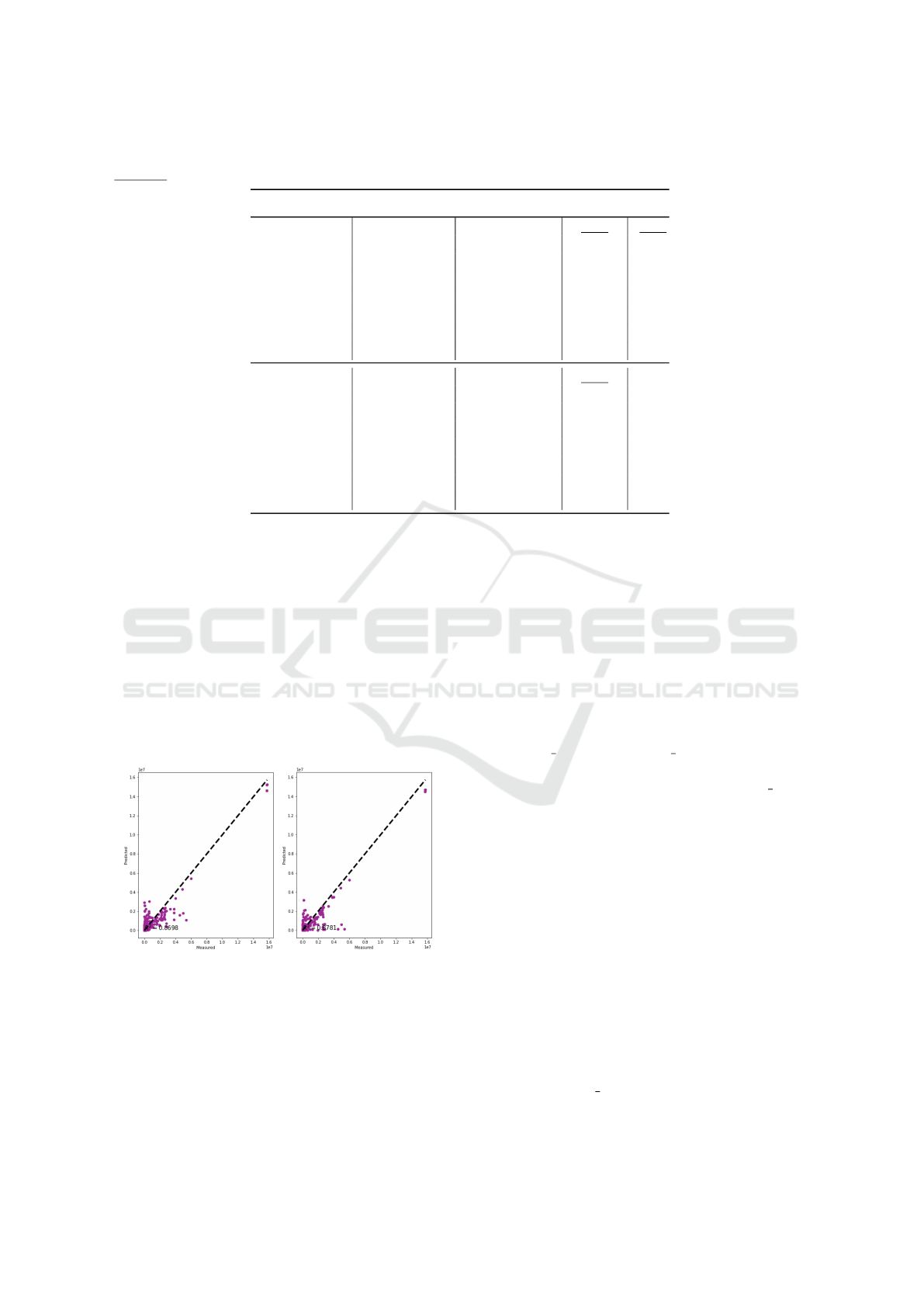
Table 2: Median prediction results for RW iterations (best values per preprocessing method in bold; best global value is
underline; the selected model is signaled by using a bold and italic font).
Preprocessing Model Name Total Time(s) NMAE R
2
IDF
RF 100 1.39 0.76
DT 77 1.41 0.67
XB 359 1.48 0.68
HGBM 1727 1.65 0.68
ET 95 1.48 0.72
SVM 147 2.33 -0.08
LSVM 88 2.32 -0.09
LGM 128 1.61 0.67
PCP
RF 870 1.36 0.65
DT 68 1.43 0.63
XB 592 1.45 0.70
HGBM 2016 1.88 0.48
ET 1204 1.42 0.63
SVM 1037 2.30 -0.08
LSVM 65 2.49 -0.15
LGM 91 1.85 0.47
For demonstration purposes, Figure 3 shows the
regression scatter plot for the IDF and PCP transforms
that was obtained during the u = 7th RW iteration
and for the RF algorithm. Each plot shows the tar-
get measured values (x-axis) versus the obtained RF
predictions (y-axis), where the dashed diagonal de-
notes the perfect regression line. Thus, the closer are
the predicted points (purple points) to the diagonal
line, the better are the predictions and the higher is
the R
2
score. For this iteration (u=7), both IDF and
PCP transforms provided a high quality result when
using the RF algorithm, resulting in very similar R
2
values (0.87 for IDF and 0.88 for PCP).
Figure 3: R
2
for RF and RW iteration u = 7, using IDF (left)
and PCP (right).
In order to select the best RUL prediction method,
we also consider the computational effort. As shown
in Table 2, the IDF based RF model requires much
less effort (it is around 8.7 times faster) when com-
pared with its PCP variant. Given that the IDF
RF combination also provided the higher median R
2
score (0.76) and second lowest NMAE median value
(1.39%), it was considered the best ML approach as
measured when using the RW evaluation.
Next, we have applied the XAI approach to the
selected ML model (IDF categorical transform and
RF algorithm). In particular, the SHAP method, by
means of the Shapash Python tool, was executed for
the IDF based RF model that was fit during the u = 7th
RW iteration. The top of Figure 4 displays the over-
all feature importance for the trained model. There is
a clear dominance of the impact of equipment-related
attributes on the expected lifetime of a spare part (e.g.,
equipment type, equipment subtype), represent-
ing approximately 80% of the total variable input in-
fluence. In contrast, the suppliers (supplier code)
have an almost irrelevant impact on the RUL forecast-
ing process, which may be explained due to the high
unavailability of data for this data field.
An additional explanatory knowledge that can be
provided by analyzing the SHAP method results in
terms of the behavior produced by changing a par-
ticular input factor in the predictions. Under an in-
teractive process, the maintenance manager can per-
form several root-cause analyses by executing distinct
what-if queries or even a full sensitivity analysis for
a particular RUL spare part prediction. For demon-
stration purposes, we exemplify a a sensitivity analy-
sis for the IDF based RF model trained during itera-
tion u=7 (bottom of Figure 4). In this visualization,
we selected a specific spare part RUL prediction, fix-
ing all input variables except the maintenance techni-
cian (technician name), which was varied through
its range. Then, the obtained SHAP contribution val-
ICAART 2022 - 14th International Conference on Agents and Artificial Intelligence
770

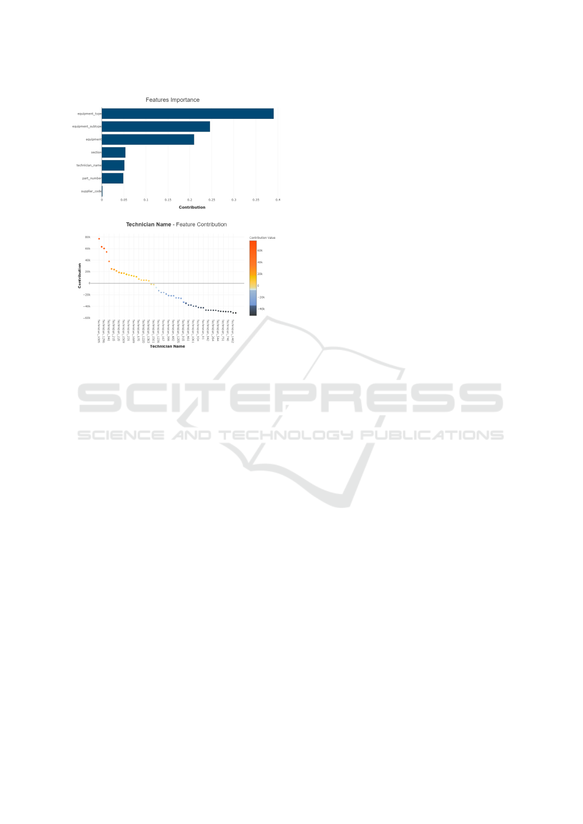
Figure 4: XAI analysis (top – importance of the input fea-
tures; bottom – sensitivity analysis for a RUL prediction).
ues (in the y-axis) were sorted in a decreasing order.
As shown in the bottom of Figure 4, there are some
technicians (e.g., #1005, #1296), that produce a posi-
tive impact in the RUL, while others tend to decrease
the RUL value (e.g., #740, #1482). This extracted
knowledge can be used by the manager to support
her/his decisions when selecting technicians to per-
form new maintenance operations. Thus, the SHAP
extracted explanatory knowledge can be potentially
used to minimize the failure rate in production lines,
thus improving the quality of the products and ser-
vices provided, and reduce the overall maintenance
activities costs.
4 CONCLUSIONS
In this work, we assume a novel data-driven RUL
prediction approach that only uses corrective mainte-
nance historical records, which are commonly avail-
able in assembly industries and thus more easy to
collect when compared with specific equipment mea-
surements that require dedicated sensors (e.g., tem-
perature levels). As a case study, we address 18,355
records with RUL measurements that were extracted
from an automotive multimedia assembly company.
Assuming a regression task, where we predict the
RUL in terms of number of produced units, we com-
pare two categorical input transforms (IDF and PCP)
and eight ML algorithms (DT, RF, ET, XG, LGBM,
HGBM, LSVM and SVM). The experimental evalu-
ation assumed a realistic and robust RW evaluation.
Overall, high-quality RUL prediction results were ob-
tained by the IDF input transform when combined
with the RF algorithm, obtaining a median NMAE
of 1.39% and median R
2
score of 0.76. This ML
approach also required a reasonable amount of com-
putational effort, being much faster when compared
with the PCP RF variant. The selected model was
further analyzed by using the SHAP XAI method for
a better understanding in preventing the occurrence of
spare part breakdowns. In particular, we have shown
how the XAI can be used to extract the relative impor-
tance of the input features and also perform a sensi-
tivity analysis, measuring the prediction model effect
of changing a selected input variable.
The obtained results were provided to the assem-
bly company maintenance experts, which provided
very positive feedback. In particular, the experts val-
ued the high predictive results (NMAE and R
2
values)
and the XAI examples. In future work, we intend to
implement the proposed IDF based RF algorithm in
a real industrial environment, using a friendly inter-
active tool (e.g., for the XAI analyses) that would al-
low us to obtain additional valuable feedback on the
usefulness of the proposed ML approach to enhance
maintenance management decisions.
ACKNOWLEDGMENTS
This work has been supported by FCT – Fundac¸
˜
ao
para a Ci
ˆ
encia e Tecnologia within the R&D Units
Project Scope: UIDB/00319/2020.
REFERENCES
Borgi, T., Hidri, A., Neef, B., and Naceur, M. S. (2017).
Data analytics for predictive maintenance of indus-
trial robots. In 2017 International Conference on Ad-
vanced Systems and Electric Technologies (IC ASET),
pages 412–417.
Breiman, L. (2001). Random forests. Machine Learning,
45(1):5–32.
Carvalho, T. P., Soares, F. A. A. M. N., Vita, R., da P. Fran-
cisco, R., Basto, J. P., and Alcal
´
a, S. G. S. (2019). A
systematic literature review of machine learning meth-
ods applied to predictive maintenance. Computers &
Industrial Engineering, 137:106024.
Chen, T. and Guestrin, C. (2016). Xgboost: A scalable tree
boosting system. CoRR, abs/1603.02754.
A Machine Learning Approach for Spare Parts Lifetime Estimation
771

Cheng, C., Ma, G., Zhang, Y., Sun, M., Teng, F., Ding,
H., and Yuan, Y. (2020). A deep learning-based re-
maining useful life prediction approach for bearings.
IEEE/ASME Transactions on Mechatronics, PP.
Cristianini, N. and Shawe-Taylor, J. (2000). Support Vector
Machines. Cambridge University Press.
Fan, Y., Nowaczyk, S., and Rognvaldsson, T. (2015). Eval-
uation of self-organized approach for predicting com-
pressor faults in a city bus fleet. Procedia Computer
Science, 53:447–456.
Geurts, P., Ernst, D., and Wehenkel, L. (2006). Extremely
randomized trees. Machine Learning, 63(1):3–42.
Goldberg, K., Roeder, T., Gupta, D., and Perkins, C. (2001).
Eigentaste: A constant time collaborative filtering al-
gorithm. Information Retrieval, 4:133–151.
Jardine, A. K., Lin, D., and Banjevic, D. (2006). A re-
view on machinery diagnostics and prognostics im-
plementing condition-based maintenance. Mechani-
cal Systems and Signal Processing, 20(7):1483–1510.
Kang, Z., Catal, C., and Tekinerdogan, B. (2021). Remain-
ing useful life (rul) prediction of equipment in pro-
duction lines using artificial neural networks. Sensors,
21(3).
Ke, G., Meng, Q., Finley, T., Wang, T., Chen, W., Ma, W.,
Ye, Q., and Liu, T.-Y. (2017). Lightgbm: A highly
efficient gradient boosting decision tree. In Proceed-
ings of the 31st International Conference on Neu-
ral Information Processing Systems, NIPS’17, page
3149–3157, Red Hook, NY, USA. Curran Associates
Inc.
Lee, S. M., Lee, D., and Kim, Y. S. (2019). The quality
management ecosystem for predictive maintenance in
the industry 4.0 era. International Journal of Quality
Innovation, 5(1):1–11.
Li, X., Zhang, W., Ma, H., Luo, Z., and Li, X. (2020).
Data alignments in machinery remaining useful life
prediction using deep adversarial neural networks.
Knowledge-Based Systems, 197:105843.
Lundberg, S. and Lee, S. (2017a). A unified approach to in-
terpreting model predictions. CoRR, abs/1705.07874.
Lundberg, S. M. and Lee, S. (2017b). A unified approach
to interpreting model predictions. In Guyon, I., von
Luxburg, U., Bengio, S., Wallach, H. M., Fergus, R.,
Vishwanathan, S. V. N., and Garnett, R., editors, Ad-
vances in Neural Information Processing Systems 30:
Annual Conference on Neural Information Processing
Systems 2017, December 4-9, 2017, Long Beach, CA,
USA, pages 4765–4774.
Matos, L. M., Cortez, P., Mendes, R., and Moreau, A.
(2018). A comparison of data-driven approaches for
mobile marketing user conversion prediction. In 2018
International Conference on Intelligent Systems (IS),
pages 140–146.
Matos, L. M., Cortez, P., Mendes, R., and Moreau, A.
(2019). Using deep learning for mobile marketing
user conversion prediction. In 2019 International
Joint Conference on Neural Networks (IJCNN), pages
1–8.
Matos, L. M., Cortez, P., and Mendes, R. C. (2020). Cane -
categorical attribute transformation environment.
Okoh, C., Roy, R., Mehnen, J., and Redding, L. (2014).
Overview of remaining useful life prediction tech-
niques in through-life engineering services. Proce-
dia CIRP, 16:158–163. Product Services Systems and
Value Creation. Proceedings of the 6th CIRP Confer-
ence on Industrial Product-Service Systems.
Oliveira, N., Cortez, P., and Areal, N. (2017). The impact of
microblogging data for stock market prediction: Us-
ing twitter to predict returns, volatility, trading vol-
ume and survey sentiment indices. Expert Syst. Appl.,
73:125–144.
Rauch, E., Linder, C., and Dallasega, P. (2020). Anthro-
pocentric perspective of production before and within
industry 4.0. Computers & Industrial Engineering,
139:105644.
Sahakyan, M., Aung, Z., and Rahwan, T. (2021). Explain-
able artificial intelligence for tabular data: A survey.
IEEE Access, 9:135392–135422.
Shalev-Shwartz, S. and Ben-David, S. (2014). Understand-
ing Machine Learning: From Theory to Algorithms.
Cambridge University Press.
Shapiro, N. Z. and Shapley, L. S. (1978). Values of large
games, I: A limit theorem. Math. Oper. Res., 3(1):1–
9.
Susto, G. A., Beghi, A., and Luca, C. (2012). A predic-
tive maintenance system for epitaxy processes based
on filtering and prediction techniques. Semiconductor
Manufacturing, IEEE Transactions on, 25:638–649.
Susto, G. A., Schirru, A., Pampuri, S., McLoone, S., and
Beghi, A. (2015). Machine learning for predictive
maintenance: A multiple classifier approach. IEEE
Transactions on Industrial Informatics, 11(3):812–
820.
Tashman, L. J. (2000). Out-of-sample tests of forecasting
accuracy: an analysis and review. International Jour-
nal of Forecasting, 16(4):437–450. The M3- Compe-
tition.
Wang, B., Lei, Y., Yan, T., Li, N., and Guo, L. (2020). Re-
current convolutional neural network: A new frame-
work for remaining useful life prediction of machin-
ery. Neurocomputing, 379:117–129.
Wang, W. (2012). An overview of the recent advances in
delay-time-based maintenance modelling. Reliability
Engineering & System Safety, 106:165–178.
Wright, S. (1921). Correlation and causation. Journal of
Agricultural Research., 20(3):557–585.
Wu, D., Jennings, C., Terpenny, J., Gao, R. X., and Kumara,
S. (2017). A Comparative Study on Machine Learn-
ing Algorithms for Smart Manufacturing: Tool Wear
Prediction Using Random Forests. Journal of Manu-
facturing Science and Engineering, 139(7). 071018.
ICAART 2022 - 14th International Conference on Agents and Artificial Intelligence
772