Vehicle Pair Activity Classiﬁcation using QTC and Long Short Term

Memory Neural Network

Rahulan Radhakrishnan

and Alaa Alzoubi

School of Computing, The University of Buckingham, Buckingham, U.K.

Keywords:

Vehicle Activity Classiﬁcation, Qualitative Trajectory Calculus, Long-Short Term Memory Neural Network,

Automatic LSTM Architecture Design, Bayesian Optimisation.

Abstract:

The automated recognition of vehicle interaction is crucial for self-driving, collision avoidance and secu-

rity surveillance applications. In this paper, we present a novel Long-Short Term Memory Neural Network

(LSTM) based method for vehicle trajectory classiﬁcation. We use Qualitative Trajectory Calculus (QTC) to

represent the relative motion between a pair of vehicles. The spatio-temporal features of the interacting vehi-

cles are captured as a sequence of QTC states and then encoded using one hot vector representation. Then,

we develop an LSTM network to classify QTC trajectories that represent vehicle pairwise activities. Most of

the high performing LSTM models are manually designed and require expertise in hyperparameter conﬁgu-

ration. We adapt Bayesian Optimisation method to ﬁnd an optimal LSTM architecture for classifying QTC

trajectories of vehicle interaction. We evaluated our method on three different datasets comprising 7257 tra-

jectories of 9 unique vehicle activities in different trafﬁc scenarios. We demonstrate that our proposed method

outperforms the state-of-the-art techniques. Further, we evaluated our approach with a combined dataset of

the three datasets and achieved an error rate of no more than 1.79%. Though, our work mainly focuses on

vehicle trajectories, the proposed method is generic and can be used on pairwise analysis of other interacting

objects.

1 INTRODUCTION

Analysing the interaction between vehicles is imper-

ative in safety critical tasks such as autonomous ve-

hicle driving. Dangerous road events such as vehi-

cle overtaking and collisions can be avoided if the

behaviours of the surrounding vehicles are captured

accurately. Vehicle activity recognition task aims

to classify the actions of one or more vehicles by

analysing their temporal sequence of observations.

Potential collisions can be avoided or minimised by

recognising the behaviour that a vehicle is in (or about

to enter) beforehand (Ohn-Bar and Trivedi, 2016). A

vehicle can have complex motion behaviours either

on its own (single activity) or with another vehicle

(pair or group activity) (Ni et al., 2009) or with sta-

tionary obstacles (e.g. stalled vehicles). In the context

of activity classiﬁcation task, two key approaches for

trajectory representation have been presented: quan-

titative and qualitative methods. Numerous studies

have been conducted using quantitative method where

https://orcid.org/0000-0002-4113-3710

https://orcid.org/0000-0003-1167-170X

real values of the features are directly used to rep-

resent the trajectories (Khosroshahi et al., 2016; Lin

et al., 2013; Deo et al., 2018). On the other hand,

qualitative methods have shown high performance for

activity classiﬁcation applications such as vehicle tra-

jectory analysis (AlZoubi et al., 2017; AlZoubi and

Nam, 2019). It has motivated the researchers to inves-

tigate qualitative representations with deep learning

methods for vehicle trajectory analysis. Qualitative

methods (e.g. QTC (Van de Weghe, 2004)) abstract

the real values of the trajectories, use symbolic rep-

resentation, are computationally less expensive, and

more human understandable than quantitative meth-

ods.

Many previous studies on both single and multi-

ple vehicle activity classiﬁcation and prediction have

deployed different techniques such as Bayesian Net-

works (Lef

evre et al., 2011) and Hidden Markov

Models (Berndt and Dietmayer, 2009; Deo et al.,

2018; Framing et al., 2018). However, the emergence

of LSTM as a powerful method to handle temporal

data with long term dependencies has increased the

interest on using such technique for vehicle activity

236

Radhakrishnan, R. and Alzoubi, A.

Vehicle Pair Activity Classiﬁcation using QTC and Long Short Term Memory Neural Network.

DOI: 10.5220/0010903500003124

In Proceedings of the 17th International Joint Conference on Computer Vision, Imaging and Computer Graphics Theory and Applications (VISIGRAPP 2022) - Volume 5: VISAPP, pages

236-247

ISBN: 978-989-758-555-5; ISSN: 2184-4321

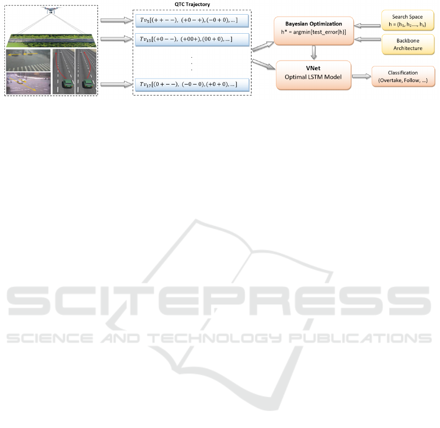
Figure 1: Our Proposed Method.

classiﬁcation task. Recently, few studies have been

proposed on using a manually designed LSTM with

quantitative methods to classify multiple vehicles ac-

tivities (Khosroshahi et al., 2016). However, incor-

porating qualitative features with LSTM for vehicle

activity analysis still remains to be an open investiga-

tion area. On the other hand, the manual design of

LSTM architectures has several limitations: 1) trial-

and-error approach is time-consuming and requires

architectural domain expertise; 2) this might result in

building an architecture that is limited to the expert

previous knowledge; and 3) error prone. In addition,

LSTM architecture has a complex structure including

gates and memory cells to store long term dependen-

cies of sequential data. Thus, it requires a methodi-

cal way of tuning its hyperparameters to get the op-

timal architecture rather than using manual designing

or brute force methods such as Grid Search and Ran-

dom Search. Bayesian Optimisation has been used

for optimising LSTM networks in applications such

as image caption generation (Snoek et al., 2015) and

forecasting (Yang et al., 2019). Such optimiser can be

adapted to design the LSTM architectures for vehicle

trajectory classiﬁcation task.

In this paper, we present our method for vehicle

pair activity classiﬁcation based on QTC and LSTM.

Our method consists of three main stages, initially

we deploy QTC to represent the relative motion be-

tween the vehicles symbolically. Then, we transform

this representation into a two-dimensional matrix us-

ing one-hot vectors. In the second stage, we em-

ploy Bayesian Optimisation approach to search for a

generic optimal Bi-LSTM architecture (to which we

refer as LSTM in this paper) for vehicle activity clas-

siﬁcation. Both model accuracy and complexity were

used as criteria in our architecture selection policy.

Finally, the optimal LSTM architecture was used to

build LSTM model (called VNet) for vehicle pair ac-

tivity recognition. Our approach was evaluated with

three publicly available datasets of vehicle interac-

tion. The results show that our proposed method out-

performs all the existing methods. Figure 1 shows an

overview of the main components of our method. Our

approach is the ﬁrst to use QTC with LSTM for pair-

wise vehicle activity classiﬁcation.

The key contributions of this paper include: (1)

We propose a new method for pair-wise vehicle ac-

tivity classiﬁcation based on QTC and LSTM net-

work; (2) We adopt Bayesian Optimisation method to

ﬁnd an optimal LSTM architecture for vehicle activ-

ity classiﬁcation with less human intervention in the

architectural and modelling design, and low risk of

model generalisation error; (3) we evidence the over-

all generality of our method with evaluations on three

vehicle interaction datasets. We show experimentally

that our proposed VNet model outperforms existing

state-of-the-art methods such as (AlZoubi and Nam,

2019; AlZoubi et al., 2017; Lin et al., 2013; Lin et al.,

2010; Ni et al., 2009; Zhou et al., 2008).

2 BACKGROUND AND

LITERATURE REVIEW

2.1 Qualitative Trajectory Calculus

Qualitative Trajectory Calculus (QTC) is a method to

represent an interaction between two moving objects

in a symbolic way (Van de Weghe, 2004). QTC con-

sists of six codes representing four features of a rel-

ative interaction: distance (C1,C2), speed (C3), side

(C4,C5) and angle (C6). These codes are represented

using three symbols: “-”, “0” and “+”. Given the po-

sitions of two moving objects (O

and O

• C1: distance of O

with respect to O

: “-” indi-

cates decrease, “+” indicates increase, and “0” in-

dicates no change;

• C2: distance of O

with respect to O

;

• C3: relative speed of O

with respect to O

at time

• C4: shifting of O

with respect to the reference

line Li that connects the two objects: “-” if it

moves to the left, “+” if it moves to the right, and

“0” if it moves along Li or stationary;

Vehicle Pair Activity Classiﬁcation using QTC and Long Short Term Memory Neural Network

237

• C5: shifting of O

with respect to Li;

• C6: the angles (e) between the velocity vectors of

the objects and vector Li: “-” if e

< e

, “+” if

> e

and “0” if e

= e

Two main variants of QTC have been proposed: Dou-

ble Cross QTC (QTC

- uses C1,C2,C3 and C4) and

Full QTC (QTC

Full

- uses all six codes). There are

81 (3

) possible states for QTC

to represent the in-

teraction in a trajectory. Even though there are 729

) possible combinations of states for QTC

Full

, only

305 states are possible in real life interaction (Van de

Weghe, 2004). For example, one object cannot move

faster than the other object when both of them are

stationary (0, 0, 0, 0, +, 0). Lately, QTC has shown

to be outperforming the quantitative methods as an

adequate trajectory representation for vehicle activ-

ity analysis task (AlZoubi and Nam, 2019; AlZoubi

et al., 2017).

2.2 Long Short-Term Memory

Long Short-Term Memory (LSTM) is an architec-

ture used in the ﬁeld of deep learning for classify-

ing and predicting time series data (Hochreiter and

Schmidhuber, 1997), and represents the state-of-the-

art method for analysing sequential data. LSTM cell

consists of a memory cell and three gates namely for-

get gate, input gate and output gate. This architec-

ture allows these cells to capture and store long term

dependencies in lengthy sequential data (Yu et al.,

2019). In recent years, deep learning neural net-

works, in particular LSTM networks, have showed

outstanding performance in a variety of sequential

data recognition and prediction applications such as

human trajectory prediction (Alahi et al., 2016; Xue

et al., 2018), time series forecasting and classiﬁcation

(Siami-Namini et al., 2019; Karim et al., 2017), nat-

ural language modelling (Sundermeyer et al., 2012),

sequence labelling (Reimers and Gurevych, 2017)

and speech synthesis (Fan et al., 2014). Bidirec-

tional LSTM (Bi-LSTM) is a variant of LSTM which

contains two LSTM layers where one of them learns

the sequential data in forward direction and the other

learns it from the backward direction (Graves et al.,

2013). It performs better than its unidirectional vari-

ant since it gets access to both past and future infor-

mation simultaneously (Siami-Namini et al., 2019).

Thus, we use the bidirectional variant of the LSTM in

our approach. Developing LSTM classiﬁers for a spe-

ciﬁc task (or application) involves designing of net-

work architecture and training parameters. Two main

approaches are followed for LSTM architecture de-

signing: manually designed (or handcraft) architec-

tures and automatically searched architectures. How-

ever, manual designing of LSTM architecture of many

hyperparameters requires expertise and time. It might

result in complex architectures and increase the risk

of model overﬁtting.

2.3 Bayesian Optimisation

Deep learning methods (e.g. Deep Convolutional

Neural Networks and Long Short-Term Memory)

have exhibited high performance in image classiﬁ-

cation and sequential data analysis for various ap-

plications. However, most of these CNNs and

LSTMs architectures have been designed and opti-

mized manually. On the other hand, Neural Archi-

tecture Search (NAS) and Hyperparameter Optimisa-

tion (HPO) are two different approaches to perform

architecture search and both have signiﬁcant overlaps

(Elsken et al., 2019). NAS and advanced NAS (Efﬁ-

cient Neural Architecture Search - ENAS) approaches

are mainly used to build architectures of DCNN for

image classiﬁcation task. ENAS has shown to be

successful in different image classiﬁcation tasks such

as medical image classiﬁcation (Ahmed et al., 2020)

and object recognition in natural images (Pham et al.,

2018).

Bayesian Optimisation is one of the recent de-

velopment in optimising deep learning hyperparame-

ters including Deep Convolutional Neural Networks

(DCNN) and LSTM. Unlike ENAS, Bayesian Op-

timisation accounts for modelling-hyperparameters

(e.g. mini-batch size, number of epochs). Bayesian

Optimisation works under the principle of Bayes the-

orem using two key elements: Acquisition Function

and Surrogate Model. The acquisition function de-

termines the next point of the search by calculating

the utility of different points in the search space. Ex-

pected Improvement is a type of the acquisition func-

tion which considers both mean and variance of the

posterior model while selecting the next hyperparam-

eter setting (Frazier, 2018). It provides the blend of

both exploration and exploitation which ensures the

optimiser does not settle for a local optima (Gelbart

et al., 2014). The surrogate model updates itself after

each iteration by ﬁtting the newly observed point of

the objective function using Gaussian Process. Few

attempts have been made to use this method to ﬁnd

optimal LSTM architectures (Snoek et al., 2015; Yang

et al., 2019; Kaselimi et al., 2019). However, no

LSTMs have been designed and optimised automat-

ically for pair vehicle activity classiﬁcation task.

VISAPP 2022 - 17th International Conference on Computer Vision Theory and Applications

238

2.4 Vehicle Trajectory Analysis

Methods for vehicle trajectory analysis can be

grouped into three categories: single-vehicle activ-

ities (Khosroshahi et al., 2016; Zyner et al., 2018;

Altch

e and de La Fortelle, 2017), pair vehicle ac-

tivities (AlZoubi et al., 2017; AlZoubi. and Nam.,

2019; AlZoubi and Nam, 2019; Zhou et al., 2008),

and group vehicle activities (Deo and Trivedi, 2018;

Lin et al., 2013; Kim et al., 2017), and a review is pro-

vided in (Ahmed et al., 2018). The spatio-temporal

representation of motion information is the ﬁrst step

in the trajectory analysis. Both quantitative (Khos-

roshahi et al., 2016; Lin et al., 2013; Deo et al., 2018)

and qualitative (AlZoubi et al., 2017; AlZoubi. and

Nam., 2019; AlZoubi and Nam, 2019) methods were

used to encode vehicle activities successfully. Khos-

roshahi et al. (Khosroshahi et al., 2016) and Philips et

al. (Phillips et al., 2017) presented manually designed

LSTM networks with quantitative features (linear and

angular changes) to classify single vehicle activities at

intersections. Both studies demonstrated the impor-

tance of ﬁnding the optimal LSTM hyperparameters

such as the number of LSTM layers and the number of

neurons per layer in achieving higher accuracy. Zyner

et al. conducted a similar study in maneuver classiﬁ-

cation of single vehicle activities in an unsignalised

intersection using x,y position coordinates, heading

angle and speed as quantitative input features (Zyner

et al., 2018). Studies of Lin et al. (Lin et al., 2013)

and Deo et al. (Deo and Trivedi, 2018; Deo et al.,

2018) focus on classifying pair-wise vehicle activi-

ties. Lin et al. (Lin et al., 2013) used a surveillance

camera dataset and showed that their heat map repre-

sentation of vehicle trajectories can achieve a classi-

ﬁcation error rate as low as 4.2%. A Hidden Markov

Model (HMM) based classiﬁcation method was de-

veloped by (Deo et al., 2018) using x, y ground plane

coordinates and instantaneous velocities in the x and

y directions as features to classify pair vehicle ma-

neuvers on a highway. Their HMM model achieved

a classiﬁcation accuracy of 87.19%. The ﬁrst method

on pair activity classiﬁcation was presented by Zhou

et al. using causality and feedback ratio (Zhou et al.,

2008). However, it was developed for human pair ac-

tivity classiﬁcation. They used Support Vector Ma-

chine (SVM) as their classiﬁer and achieved 92.1%

accuracy in classifying human pair activities. This

method has also been used by Lin et al. (Lin et al.,

2013) for vehicle activity classiﬁcation.

Unlike quantitative methods, only few studies

have been conducted on qualitative features for ve-

hicle trajectory analysis. Initial investigation on qual-

itative methods were conducted by (AlZoubi et al.,

2017). They deployed QTC as the qualitative fea-

ture extraction technique. AlZoubi et al. used the

Surveillance Camera dataset which was previously

used in the heat map based vehicle trajectory clas-

siﬁcation algorithm (Lin et al., 2013) and reduced

the classiﬁcation error rate up to 3.44%. Hence,

showed that their QTC method outperforms the quan-

titative heat map method for classiﬁcation of vehi-

cle trajectories. Further, they expanded their study

and developed a DCNN method (TrajNet) to clas-

sify QTC sequences and achieved a reduced classiﬁ-

cation error rate of 1.16% from the same dataset (Al-

Zoubi and Nam, 2019). TrajNet maps the QTC tra-

jectory into image texture and uses transfer learning

with AlexNet CNN model for activity classiﬁcation.

The same authors also developed a simulation dataset

with three classes including collision scenarios (Al-

Zoubi and Nam, 2019). However, none of the afore-

mentioned techniques have investigated the incorpo-

ration of QTC and LSTM to solve this problem. It is

worth mentioning that one attempt was made to use

both QTC and manually designed LSTM architecture

for gaming application (Panzner and Cimiano, 2016).

The architecture contains a single LSTM layer with

128 hidden units without any dropout. This study

showed the potential of using QTC with manually de-

signed LSTM. However, LSTM is yet to be used with

qualitative features such as QTC in the context of ve-

hicle trajectory analysis.

We adopt the quantitative methods (AlZoubi et al.,

2017; Lin et al., 2013; Lin et al., 2010; Ni et al., 2009;

Zhou et al., 2008) and the qualitative method (Al-

Zoubi and Nam, 2019) as benchmark techniques for

our study, against which we evaluate our work. In ad-

dition, we also compare the performance of the man-

ually designed LSTM architecture in (Panzner and

Cimiano, 2016) against our optimised LSTM archi-

tecture.

3 PROPOSED METHOD

The proposed method comprises of three main com-

ponents: 1) Representing pair-wise vehicle move-

ments as QTC trajectory sequences; 2) Searching for

optimal LSTM architecture using Bayesian Optimisa-

tion method; and 3) Developing LSTM model (VNet)

for classifying QTC trajectories of interacting vehi-

cles. Our method for classifying vehicle trajectories

involves generation of QTC trajectories, automatic

designing of LSTM architecture with optimised mod-

elling hyperparameters, learned from the data, and ac-

counts for signiﬁcant differences in sequence length

and interaction complexity. As presented in Section 4,

Vehicle Pair Activity Classiﬁcation using QTC and Long Short Term Memory Neural Network

239

our method generalises across three different vehi-

cle interaction datasets, and enables us to consistently

outperform state-of-the-art vehicle pair-activity anal-

ysis methods.

3.1 QTC Trajectory Generation and

Representation

The 2D position coordinates x;y are used to represent

the relative motion between two vehicles, and encode

their interaction as a trajectory of QTC states. In this

study, we use both QTC

and QTC

Full

variants de-

rived directly using the vehicle centre position coor-

dinates.

Deﬁnition: Given two interacting vehicles with their

x; y position coordinates during the time interval t

, the trajectories of the two vehicles are deﬁned as:

V 1

= {(x

, y

), ..., (x

, y

), ..., (x

, y

);

V 2

= {(x

, y

), ..., (x

, y

), ..., (x

, y

where (x

) is the position coordinates of the ﬁrst

interacting vehicle at time t, (x

) is the position co-

ordinates of the second, and k is the total number of

time steps in the trajectories. The pair-wise trajec-

tory is deﬁned as a sequence of corresponding QTC

states: T v

= {S

, ..., S

, ...S

}, where S

is the QTC

state representation of the relative movement of the

two vehicles between time t and t +1 in trajectory T v

and N is the number of QTC observations (N = k −1)

in T v

. Due to the limited computational resources,

we used QTC

variant for the architecture search and

modelling as described in Section 3.2, while QTC

Full

was only used for modelling.

QTC Trajectory to One Hot Vector Representa-

tion: The trajectory T v

is a time varying, one dimen-

sional sequence of QTC states and it is represented as

a sequence of characters Ch

= {Ch

, ...,Ch

, ...Ch

}

in a text format. This text format only provides the

presence of a QTC state (Character) at a particular

time. Thus, it loses the information of QTC states

which are absent in that time frame. To capture this

high level information, the QTC sequence of charac-

ters (Ch

) were translated into numerical format using

One Hot encoding without losing its location informa-

tion. Thus, the one hot vector representation of trajec-

tory T v

provides a 2D matrix (Mv

) of size (Q ∗ N);

where Q is the number of possible QTC states and

N is the number of observations in T v

. This matrix

is used as the sequential input for the LSTM model

presented in Section 3.2.

3.2 Vehicle Activity Classiﬁcation

In this section, we present the formulation of our

LSTM architecture with QTC trajectories for vehicle

activity classiﬁcation. Gaining inspiration from au-

tomatic network search, we aim to take advantage of

Bayesian Optimisation method which is a powerful

technique to optimise deep learning hyperparameters.

First, we deﬁne an LSTM backbone architecture and

targeted hyperparameter search space. Then, we em-

ploy Bayesian Optimisation to ﬁnd the optimal archi-

tecture and training parameters for accurate vehicle

activity classiﬁcation.

3.2.1 Backbone Architecture Design and Search

Space

Bayesian Optimisation requires a deﬁnition of ini-

tial backbone architecture and the trainable hyper-

parameters. We designed a backbone architecture

consisting six layers: Sequence Input Layer (SI),

Bi-directional LSTM Layer (LST M), Dropout Layer

(DL), Fully Connected Layer (FL), SoftMax Layer

(SM), and Classiﬁcation Layer (OL) in sequential or-

der as shown in Figure 2. Based on the pair-wise

vehicle trajectory representation (one hot vector) in

Section 3.1, an input layer was deﬁned with size

(Q∗N). This was followed by L number of (Bi-LSTM

+ Dropout) Layer Pairs where m is the number of hid-

den units of the Bi-LSTM Layer and p is the dropout

percentage of the dropout layer. Values of L, m and

p were determined by the Bayesian Optimisation al-

gorithm. Our method identify the values of m and p

for each L (i.e. if we have two layers L = 2, m and p

values of each layer are estimated: (m

), (p

)).

Then, a fully connected layer was added based on the

number of vehicle activity classes C in the dataset. Fi-

nally, a softmax layer and classiﬁcation output layer

were incorporated to match the number of classes C.

The softmax layer produces a probability distribution

over all the class labels. The output of the softmax

layer is passed to a classiﬁcation layer which com-

putes the cross-entropy loss of each class to measure

the performance of the classiﬁcation.

The selection of suitable hyperparameter search

space for building LSTM network plays a major role

in the model performance. We deﬁned six hyper-

parameters for tuning our LSTM for vehicle trajec-

tory classiﬁcation. The search space boundaries of

the identiﬁed optimisable hyperparameters are: L

= {1, 2, 3}, m = [8 − 512], p = {0, 25, 50, 75}%,

Epochs (E po) = [1 − 400], Minibatch Size (MB)

= {2, 4, 8, 16}, Optimiser (Opt) = {SGDM, Adam,

RMSprop}. The search space (values, boundaries and

categories) of the above mentioned hyperparamters

were selected based on two criteria: the best perform-

ing hyperparameters of previous studies (Reimers and

Gurevych, 2017) and suitability for our vehicle’s ac-

tivity classiﬁcation task.

VISAPP 2022 - 17th International Conference on Computer Vision Theory and Applications

240

Figure 2: Proposed LSTM Backbone Architecture.

3.2.2 Automatic Architecture Search

Given the backbone architecture and the search space

hyperparameters h, we use Bayesian Optimisation

method to ﬁnd the optimal values of L, m, p, E po, MB,

and Opt. Thus, h = {h

, ..., h

} where h

the value of optimisable hyperparameter j in hyper-

parameter setting h and z is the total number of hy-

perparameters that are being optimised (in this case

z = 6). Firstly, we deﬁne the objective function f (h)

which we want the Bayesian Optimiser to minimize.

The objective function, f (h) is deﬁned as the classi-

ﬁcation error rate of the test set when modelling the

backbone architecture with hyperparameter setting h:

f (h) = Classiﬁcation Error(h) (1)

Number of seed points (r) that the Bayesian Opti-

miser uses to create the surrogate model was set to

4 and the number of search iterations was selected as

30. Those values were selected empirically. Num-

ber of seed points deﬁnes the number of points that

the Bayesian Optimiser examines before starting the

search process. Bayesian Optimiser uses those 4 seed

points to build the surrogate model and then iterates

30 times to select the optimal architecture. Initially,

Bayesian Optimiser randomly selects 4 sets of hy-

perparameter settings as the initial seed points and

models the backbone architecture using each of those

four settings. Then, it calculates the test error rate of

those four models to create the surrogate model G(h).

Gaussian Process Model (Regression) is used to con-

struct the surrogate model. After creating the surro-

gate model, Bayesian Optimiser selects a new hyper-

parameter setting using an acquisition function. We

use the acquisition function Expected Improvement

EI(h) which selects the next hyperparameter setting

as the one that has the highest expected improvement

over the current best observed point (lowest classiﬁ-

cation error) of the objective function. The Expected

Improvement for hyperparameter setting h is,

EI(h) = E(max( f

∗

(h) − G(h), 0)) (2)

where G(h) is the current posterior distribution of the

surrogate model and f

∗

(h) is best observed point of

Algorithm 1: Bayesian Optimisation.

Input: Hyperparameter Seach Space h

Input: Objective Function f (h)

Input: Max No of Evaluation n

max

Input: Initial Seed Points r

Output: Optimal hyperparameter setting h

∗

Output: Classiﬁcation Error of Optimal hyperpa-

rameter setting d

∗

Select: initial hyperparameter settings h

∈ h for r

number of points

Evaluate: the initial classiﬁcation error d

= f (h

)

Set h

∗

= h

and d

∗

= d

for n = 1 to n

max

Select: a new hyperparameter conﬁguration h

∈ h

by optimising the acquisition function D(h

)

= argmax(D(h

))

where,

D(h

) = EI(h

) = E(max( f

∗

(h) − G(h

), 0))

Evaluate: f for h

to obtain the classiﬁcation error

= f (h

) for hyperparameter setting h

Update: the surrogate model

if d

∗

then h

∗

= h

and d

∗

= d

end if

end for

Output: h

∗

and d

∗

the objective function so far. The h which maximizes

the acquisition function is evaluated next and the sur-

rogate model gets updated with this newly evaluated

point. This process repeats until a ﬁxed number of it-

erations (n

max

= 30 iterations). Algorithm 1 elaborates

this process in detail.

3.2.3 Optimal Architecture Selection and

Modelling

We used two real-world datasets to identify a generic

optimal architecture for vehicle activity classiﬁcation.

As described in Section 4, each vehicle trajectory

dataset was split into 5 groups (5-folds cross vali-

Vehicle Pair Activity Classiﬁcation using QTC and Long Short Term Memory Neural Network

241

dation). The selection of the optimal architecture

was carried out under two stages: initially within

the dataset and then between the datasets. In the

ﬁrst stage, we generated 150 LSTM architectures per

dataset (i.e. 30 architectures per fold) using Bayesian

Optimisation. We deﬁned two selection criteria: 1)

low classiﬁcation error; and 2) low architecture com-

plexity. First, from each dataset, the architectures

which provide the lowest classiﬁcation error on the

test set were selected from each fold. Then, the best

architecture of each fold was selected by comparing

their complexities. Complexity of the architecture is

determined by the total number of trainable param-

eters (T.P). Our proposed architecture consists train-

able parameters from Bi-LSTM layer and Fully Con-

nected layer which can be calculated using equation

T.P = 2(4m(Q + m + 1)) +C(2m + 1) (3)

where 4 represents the 4 activation function unit equa-

tions of the LSTM cell and 2 represents the Bi-LSTM

variant of the LSTM. The ﬁrst stage of selection re-

sults in the best 5 architectures from each dataset. In

the second stage, we compare the similarities of the

best architectures between the datasets. We use a sim-

ple similarity measure which is determined by how

identical (or similar) the values of hyperparameters

(L, m and p) are between two architectures from the

two datasets. Using this similarity measure, we iden-

tify a generic optimal architecture suitable for vehicle

activities observed from different settings. Our moti-

vation behind this approach of searching for optimal

architectures from two datasets separately was identi-

fying one generic architecture applicable for different

vehicle activity datasets as illustrated in Section 4.

Given the one hot vector representation of pair vehi-

cle trajectories and the optimal architecture, we build

VNet models for different activity classiﬁcation. The

fully connected layer of the optimal architecture was

updated according to the number of classes C in the

dataset.

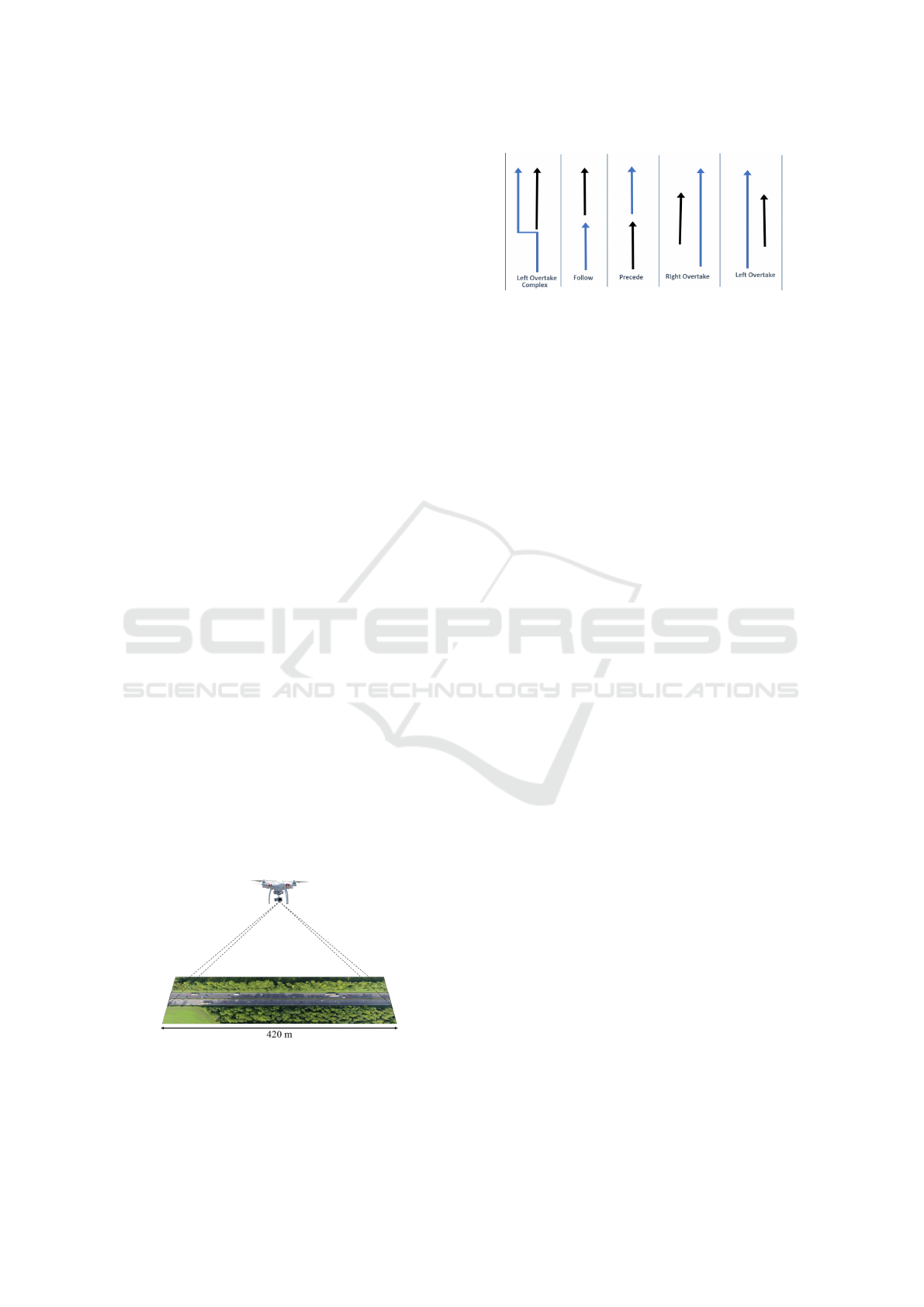
Figure 3: Example of Moving Vehicles Captured from a

Drone Camera for HighD Dataset (Krajewski et al., 2018).

Figure 4: Example Pair-wise Manoeuvres of HighD dataset

(Krajewski et al., 2018).

4 DATASETS AND

EXPERIMENTS

This section presents three publicly available vehi-

cle interaction datasets and comparative experiments

to evaluate the effectiveness of our method. All ex-

periments were conducted on an Intel Core i7 lap-

top, CPU@1.80GHz with 8.0GB RAM. All three

datasets were captured in different settings and con-

sist of different types of vehicle interactions. Fur-

ther, we developed a challenging fourth dataset which

combined all three datasets to evaluate our generic

LSTM model. Finally, we evaluated an existing man-

ually designed LSTM developed for QTC to deter-

mine the importance of incorporating automatic op-

timisation of LSTM architecture for vehicles activity

analysis domain.

Dataset 1: Highway Drone Dataset: Highway

Drone (HighD) Dataset is a dataset of vehicle trajec-

tories recorded using a drone (Krajewski et al., 2018).

Figure 3 shows the placement of the drone camera in

the data collection region. The dataset consists tra-

jectories of more than 110,500 vehicles with their x, y

position coordinates at each timestamp. Five unique

vehicle pair activities (Follow, Precede, Left Over-

take, Left Overtake (Complex) and Right Overtake)

were extracted from the dataset as illustrated in Fig-

ure 4. Follow and Precede are deﬁned as Eco vehi-

cle is followed or preceded by another vehicle. Simi-

larly, Left Overtake and Right Overtake are annotated

as Eco vehicle is overtaken by another vehicle on the

left or right lane. Left Overtake (Complex) is a com-

bination of two behaviours. Initially, the Eco vehicle

is followed by another vehicle on the same lane and

then it is successfully overtaken by that vehicle using

the left lane. 6805 trajectories (1361 trajectories per

class) were selected from the dataset in order to avoid

imbalance between the classes and due to the limited

computational resource to model the LSTM network.

The dataset has sequences in varying lengths from 11-

1911 timesteps. Among the 6805 trajectories, 500

(100 trajectories per class) were used for searching

VISAPP 2022 - 17th International Conference on Computer Vision Theory and Applications

242

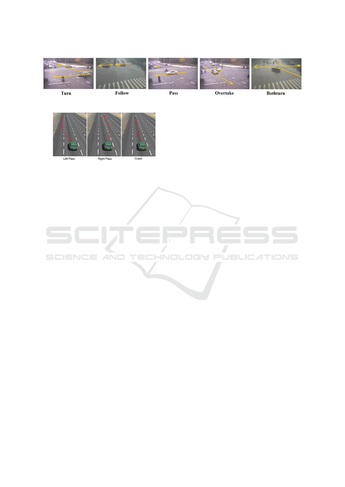
Figure 5: Example Pair-wise Manoeuvres of Trafﬁc Dataset (Lin et al., 2013).

Figure 6: Example Pair-wise Manoeuvres of VOI dataset

(Alzoubi and Nam, 2018).

the optimal architecture. On the other hand, 5000 tra-

jectories were selected from the 6805 and used for

modelling, and the remaining 1805 trajectories were

kept unseen for external testing.

Dataset 2: Trafﬁc Dataset: The trafﬁc dataset was

generated by extracting position coordinates of vehi-

cles from 20 surveillance videos (Lin et al., 2013).

The videos are recorded from a road junction using

different surveillance cameras as shown in ﬁgure 5.

The dataset contains 175 trajectories of pair vehicles

in the form of x, y positions where each trajectory has

a length of 20 time steps. It has ﬁve unique vehicle

pair activities namely Turn, Follow, Pass, Overtake

and Both Turn as shown in Figure 5, and each activity

has 35 trajectories in the dataset.

Dataset 3: Vehicle Obstacle Interaction Dataset:

Vehicle Obstacle Interaction (VOI) dataset is obtained

through a simulation environment, and it mainly

focuses on close proximity manoeuvrings and rare

events for which there are not enough real-life data

such as crash (AlZoubi. and Nam., 2019). The dataset

contains 277 pair vehicle trajectories, in the form of

x, y positions, representing three classes which are

Left Pass (104 trajectories), Right Pass (106 trajec-

tories) and Crash (67 trajectories) as shown in Figure

6. The pair trajectories has lengths ranging from 10

to 71 time steps. Left Pass and Right Pass are deﬁned

as vehicle successfully passing an obstacle on the left

or right, respectively. Crash is deﬁned as the collision

of moving vehicle with an obstacle.

Dataset 4: Combined Dataset: Combined dataset is

constructed by combining the three above mentioned

datasets with careful consideration in preserving their

ground truths while merging and splitting the com-

mon classes. Thus, this fourth dataset contains 952

trajectories with 9 classes: Follow (135), Left Pass

(138), Right Pass (107), Turn (35), Both Turn (35),

Crash (67), Preceding (100), Right Overtake (135)

and Left Overtake (200). The deﬁnition of this classes

remains the same as their original.

4.1 LSTM Architecture Optimisation

To ﬁnd the optimal hyperparameters of our proposed

backbone LSTM architecture, we perform Bayesian

Optimisation on the two real world datasets (High-

way Drone and Trafﬁc datasets). Firstly, both datasets

were divided into 5 non-overlapping folds of train-

ing and testing (5-fold cross validation protocol). In

addition, the optimisable hyperparameters and their

search space (Section 3.2.1) were provided as input

for the optimiser. The error rate of the test set of

each fold has been determined as the objective func-

tion. 150 search iterations (30 iterations per fold)

were performed individually on both datasets. Our

selection method (Section 3.2.3) was used to iden-

tify the optimal and generic architecture. The ar-

chitectures with the lowest testing error rate in each

fold were selected. HighD Dataset provided 47 archi-

tectures with highest testing accuracy. On the other

hand, the Trafﬁc dataset provided only 6 architectures

with highest testing accuracy. Since there were nu-

merous architectures that achieved the highest fold

wise accuracy, we compared their architecture com-

plexity to select the best one from each fold. The

summary of the best models of HighD and Trafﬁc

datasets from each fold are presented in Table 1. The

selected architectures of Models 2, 3 and 4 provided

the best classiﬁcation accuracy and the best class wise

standard deviation among the ﬁve models of HighD

dataset. Model 2 provided the best accuracy (93.88%)

for Trafﬁc dataset. Our aim was to ﬁnd a single op-

timal architecture for vehicle activity classiﬁcation

from both datasets. Thus, we compared the similar-

ities of the best performing architectures of both the

datasets. Model 2 of both datasets have produced ex-

actly the same LSTM architecture with slight differ-

ences in the mini batch size and number of epochs.

Those two architectures share the same L, m and p

hyperparameters. Therefore, we selected this archi-

tecture as our generic optimal architecture. We used

Vehicle Pair Activity Classiﬁcation using QTC and Long Short Term Memory Neural Network

243

Table 1: Summary of the Best Performing Architectures: D.S - Dataset, Arc - Architecture Acc - Accuracy, S.D - Class-wise

Standard Deviation, T.Par - Trainable Parameters, Opt - Optimiser, L - Number of (Bi-LSTM + Dropout) Layer Pairs, m -

Number of Hidden Units, p - Dropout Percentage, MB - Mini Batch Size, Epo - Number of Epochs.

D.S Arc Acc(%) S.D T.Par Opt L m p MB Epo

HighD

1 99.00 2.24 9149 RMSprop 1 12 25% 8 23

2 100.00 0.00 93097 sgdm 1 74 50% 8 232

3 100.00 0.00 184909 adam 1 116 0% 8 381

4 100.00 0.00 36865 sgdm 1 38 50% 8 165

5 99.00 2.24 23819 sgdm 1 27 0% 16 379

Trafﬁc

1 91.84 11.25 35749 sgdm 1 37 25% 8 283

2 93.88 11.25 93395 sgdm 1 74 50% 4 376

3 89.80 10.81 28465 sgdm 1 31 75% 4 372

4 91.84 11.25 187909 sgdm 1 117 75% 8 395

5 85.71 31.94 5879 sgdm 1 8 50% 8 69

the modelling-hyperparameters (E po, MB and Opt)

of Model 2 of HighD dataset to model our VNet clas-

siﬁcation models since HighD dataset is more chal-

lenging and 25 times larger than the Trafﬁc dataset

and it has a trajectory length range from 11-1911.

4.2 Evaluation of the Optimal

Architecture

In this section, we evaluated the selected optimal ar-

chitecture (Section 4.1) using all three datasets as well

as the combined dataset. To determine the classiﬁ-

cation error rates using our method, we used 5-fold

cross validation. On each iteration, we split the one

hot vector representation of the trajectories extracted

from the dataset into training and testing sets at ratio

of 80% to 20%, for each class. The training sets were

used to parametrise our LSTM network. The test set

was then classiﬁed by our trained VNet models.

4.2.1 Classiﬁcation of Highway Drone Dataset

Using the one hot vector representations of the 5000

trajectories extracted from HighD dataset, the VNet

model was able to classify the HighD dataset with

an average accuracy of 99.80% (std=0.35%) on the

5 folds during the modelling. We evaluated the

model using both QTC

and QTC

Full

and it achieved

the same results. Further, we tested the 5 trained

VNet models on the 1805 trajectories of unseen

dataset, achieving an average accuracy of 99.87%

(std=0.29%). Even though only 10% of the whole

dataset was used to ﬁnd the optimal architecture, our

VNet models maintained a high performance and gen-

eralised on unseen datasets. It also shows the power

of QTC in representing pair activity trajectories. For

comparative purposes, we have used the DCNN-QTC

(‘TrajNet’) (AlZoubi and Nam, 2019) as a benchmark

qualitative method, which has itself been shown to

outperform other qualitative and quantitative methods

(AlZoubi et al., 2017; Lin et al., 2013; Lin et al., 2010;

Ni et al., 2009; Zhou et al., 2008). Using the same

HighD dataset split, our VNet achieved a higher accu-

racy against TrajNet which achieved an average accu-

racy of 98.60% on 5-fold cross validation and 98.98%

on unseen test set. The difference in accuracy of our

VNet model and TrajNet is 1.2% in 5-fold modelling.

However, this 1.2% accounts for 60 trajectories in the

HighD dataset. Our VNet model was able to correctly

classify 60 more trajectories than TrajNet. Especially,

VNet performs better than TrajNet when classifying

simple and complex activities of similar behaviours

(Left Overtake and Left Overtake Complex) (Table 2).

Thus, it shows the superiority of our model statisti-

cally in such critical application. Further, our method

shows relatively high consistency among the 5 models

by providing lower standard deviation in both mod-

elling and external testing. Table 2 shows the perfor-

mance of both VNet and TrajNet on the internal and

unseen HighD datasets.

Table 2: Comparison between Our Proposed Method with

State-of-the-art TrajNet Method on HighD Dataset: Ave.

Acc. - Average Accuracy, S.D - Standard Deviation.

Model

Modelling External Testing

VNet Trajnet VNet Trajnet

Follow 99.80% 98.00% 100% 99.34%

Left

Overtake

100% 97.00% 100% 97.40%

Left

Overtake

Complex

99.20% 98.00% 99.36% 98.44%

Preceding 100% 100% 100% 99.90%

Right

Overtake

100% 100% 100% 99.76%

Ave Acc. 99.80% 98.60% 99.87% 98.98%

S.D 0.35% 1.34% 0.29% 1.05%

VISAPP 2022 - 17th International Conference on Computer Vision Theory and Applications

244

Table 3: Average Classiﬁcation Accuracy of Different Algorithms on the Trafﬁc Dataset.

Type VNet (AlZoubi

and Nam,

2019)

(AlZoubi

et al.,

2017)

(Lin et al.,

2013)

(Zhou

et al.,

2008)

(Ni et al.,

2009)

(Lin et al.,

2010)

Turn 100% 97.10% 97.10% 97.10% 98.00% 83.10% 89.30%

Follow 100% 100% 94.30% 88.60% 77.10% 61.90% 84.60%

Pass 100% 100% 100% 100% 88.30% 82.40% 84.50%

Bothturn 97.14% 100% 97.10% 97.10% 98.80% 97.10% 95.80%

Overtake 97.14% 97.10% 94.30% 94.30% 52.90% 38.30% 63.40%

Ave. Acc. 98.86% 98.84% 96.56% 95.42% 83.02% 72.76% 83.52%

4.2.2 Classiﬁcation of Trafﬁc Dataset

We have conducted similar classiﬁcation experiments

using the trafﬁc activity dataset presented in (Lin

et al., 2013). The optimal architecture was evaluated

using 5-folds cross validation using both QTC

and

QTC

Full

and the model achieved an average accuracy

of 98.86% (std=1.56%). 5-folds cross validation pro-

tocol guarantees that every trajectory in the dataset is

tested at least once. Table 3 shows the performance

comparison of our VNet against state-of-the-art ap-

proaches on this dataset (AlZoubi and Nam, 2019; Al-

Zoubi et al., 2017; Lin et al., 2013; Lin et al., 2010; Ni

et al., 2009; Zhou et al., 2008). Our method outper-

formed all six quantitative and qualitative methods by

achieving the lowest classiﬁcation error rate of 1.14%.

4.2.3 Classiﬁcation of VOI Dataset

Classifying very dangerous vehicle interactions is

crucial for collision avoidance and security surveil-

lance applications. Therefore, to gain traction as

a mainstream analysis technique, we evaluated our

method on the publicly available VOI dataset (Al-

zoubi and Nam, 2018) of crash behaviours. Using

5-folds cross validation, our VNet model achieved a

high average accuracy with 0% error rate which is

similar to TrajNet (AlZoubi and Nam, 2019). Both

QTC

and QTC

Full

achieved the same results. De-

spite the optimal architecture was designed from dif-

ferent vehicle datasets, our VNet generalized and

achieved a high performance on the VOI dataset.

4.2.4 Classiﬁcation of Combined Dataset

Our main motivation is a generic supervised analy-

sis for vehicle interactions. The combined dataset is

challenging, as it contains simple and compound ac-

tivities and with various lengths. We split the 952 tra-

jectories into training and testing sets at ratio of 80%

to 20%, for each class. The training sets were used to

parametrise our network and the test set was then clas-

siﬁed by our trained VNet model. Our VNet achieved

an average accuracy of 98.21% on the 5 folds which

shows how well our optimal architecture is gener-

alised across different and challenging datasets. For

comparative purposes, we have used TrajNet (Al-

Zoubi and Nam, 2019) as a benchmark qualitative

method. Using the same 5-fold split, our VNet model

outperforms TrajNet (Accuracy = 98.10%). Similar

to Experiment 4.2.1, TrajNet struggles to distinguish

between similar activities of the same side such as

(Left Overtake, Left Pass) and (Right Overtake, Right

Pass). VNet clearly outperforms TrajNet in those four

activities by classifying them with an average accu-

racy of 99.52% compared to TrajNet’s 98.24%. Thus,

both Experiment 4.2.1 and 4.2.4 show that VNet per-

forms better than TrajNet in distinguishing closely

matched behaviours such as Left Overtake, Left Over-

take Complex and Left Pass.

4.2.5 Manual vs Automatic LSTM Architecture

Design

Sections 4.2.1 - 4.2.4 have shown that our method out-

performed existing quantitative and qualitative meth-

ods evaluated on different and challenging datasets.

To the best of our knowledge, no existing LSTM ar-

chitecture has been designed (manually or automat-

ically) for vehicle pair activity classiﬁcation. In or-

der to evaluate the performance of our auto-optimised

LSTM architecture, we used the manually designed

LSTM architecture developed for QTC features in

(Panzner and Cimiano, 2016) as a benchmark.

Using the same evaluation protocol, the models

of manually designed architecture achieved average

accuracies of 89.12%, 72%, 21.30%, and 26.79% on

VOI, Trafﬁc, HighD, and Combined datasets, respec-

tively. The low performance of these models is a re-

sults of poor LSTM architecture design. This shows

that careful architecture design and parameter selec-

tion is very crucial for a successful vehicle activity

classiﬁcation model. Table 4 shows the results of

the model (Panzner and Cimiano, 2016) compared

against state-of-the-art TrajNet (AlZoubi and Nam,

2019) model and our VNet model. Our VNet model

Vehicle Pair Activity Classiﬁcation using QTC and Long Short Term Memory Neural Network

245

Table 4: Average Classiﬁcation Accuracy of Manually De-

signed LSTM (Handcrafted) (Panzner and Cimiano, 2016),

TrajNet (AlZoubi and Nam, 2019) and Our VNet across all

the datasets: H.LSTM - Handcrafted LSTM, Comb. - Com-

bined Dataset.

Method HighD Trafﬁc VOI Comb.

H. LSTM 21.30% 72.00% 89.12% 26.79%

TrajNet 98.60% 98.84% 100% 98.10%

VNet 99.80% 98.86% 100% 98.21%

outperforms existing methods including the manually

optimised LSTM across all the datasets.

5 CONCLUSION

In this paper, we proposed a novel method for vehi-

cle activity classiﬁcation using QTC and LSTM. We

used a qualitative feature representation method QTC

to represent the relative motion between two objects.

We then encoded the QTC sequences into a two-

dimensional matrix using one-hot vectors. Our results

show how efﬁciently our representation has abstracted

the features from real valued trajectories. Subse-

quently, we presented a method to efﬁciently ﬁnd an

optimal LSTM architecture using Bayesian Optimi-

sation for accurate analysis of vehicle activities. Our

contribution is not only restricted to producing an op-

timal architecture for vehicle activity classiﬁcation.

We also have presented a way to select the optimal

architecture for LSTM using Bayesian Optimization.

Thus, the approach can be used for other activity

classiﬁcation applications as well. Our method has

been evaluated on three completely different datasets

recorded from different types of sources: a static cam-

era, a drone camera and a simulator. We compared

our method against the state-of-the-art qualitative (Al-

Zoubi and Nam, 2019; AlZoubi et al., 2017) and

quantitative (Lin et al., 2013; Zhou et al., 2008; Ni

et al., 2009; Lin et al., 2010) methods. The results

of the combined dataset (98.21% accuracy) evidently

show that our approach is a generalised solution for

vehicle activity classiﬁcation.

Future self-driving technologies can be beneﬁted

with our approach to tackle path planning and safety

related issues. Intrigued by the results, we intend to

extend our work by investigating on quantitative fea-

tures to use with our auto-optimised LSTM. It will lay

the foundation to evaluate both qualitative and quan-

titative approaches with deep neural networks under

the same experimental framework. We evaluated our

method on a large dataset (HighD) with 6805 tra-

jectories, however, both Trafﬁc (175) and VOI (277)

datasets are relatively small. Trajectories of Trafﬁc

dataset (Lin et al., 2013) are also limited to a ﬁxed

length of 20 timesteps. Further, other potential inter-

actions such as chasing, collision of two moving vehi-

cles are not present in the datasets we have. Thus, we

hope to include these kinds of interactions in future.

In addition, we also plan to evaluate other sequential

modeling methods such as transformers, causal and

dilated convolutional neural networks.

REFERENCES

Ahmed, M., Du, H., and AlZoubi, A. (2020). An enas

based approach for constructing deep learning models

for breast cancer recognition from ultrasound images.

arXiv preprint arXiv:2005.13695.

Ahmed, S. A., Dogra, D. P., Kar, S., and Roy, P. P.

(2018). Trajectory-based surveillance analysis: A sur-

vey. IEEE Transactions on Circuits and Systems for

Video Technology, 29(7):1985–1997.

Alahi, A., Goel, K., Ramanathan, V., Robicquet, A., Fei-

Fei, L., and Savarese, S. (2016). Social lstm: Human

trajectory prediction in crowded spaces. In Proceed-

ings of the IEEE conference on computer vision and

pattern recognition, pages 961–971.

Altch

e, F. and de La Fortelle, A. (2017). An lstm network

for highway trajectory prediction. In 2017 IEEE 20th

International Conference on Intelligent Transporta-

tion Systems (ITSC), pages 353–359.

AlZoubi, A., Al-Diri, B., Pike, T., Kleinhappel, T., and

Dickinson, P. (2017). Pair-activity analysis from video

using qualitative trajectory calculus. IEEE Transac-

tions on Circuits and Systems for Video Technology,

28(8):1850–1863.

Alzoubi, A. and Nam, D. (2018). Vehicle Obstacle Interac-

tion Dataset (VOIDataset).

AlZoubi, A. and Nam, D. (2019). Vehicle activity recogni-

tion using dcnn. In International Joint Conference on

Computer Vision, Imaging and Computer Graphics,

pages 566–588. Springer.

AlZoubi., A. and Nam., D. (2019). Vehicle activity recogni-

tion using mapped qtc trajectories. In Proceedings of

the 14th International Joint Conference on Computer

Vision, Imaging and Computer Graphics Theory and

Applications - Volume 5: VISAPP,, pages 27–38. IN-

STICC, SciTePress.

Berndt, H. and Dietmayer, K. (2009). Driver intention in-

ference with vehicle onboard sensors. In 2009 IEEE

international conference on vehicular electronics and

safety (ICVES), pages 102–107. IEEE.

Deo, N., Rangesh, A., and Trivedi, M. M. (2018). How

would surround vehicles move? a uniﬁed framework

for maneuver classiﬁcation and motion prediction.

IEEE Transactions on Intelligent Vehicles, 3(2):129–

140.

Deo, N. and Trivedi, M. M. (2018). Multi-modal trajec-

tory prediction of surrounding vehicles with maneuver

based lstms. In 2018 IEEE Intelligent Vehicles Sym-

posium (IV), pages 1179–1184. IEEE.

VISAPP 2022 - 17th International Conference on Computer Vision Theory and Applications

246

Elsken, T., Metzen, J. H., and Hutter, F. (2019). Neural

architecture search: A survey. The Journal of Machine

Learning Research, 20(1):1997–2017.

Fan, Y., Qian, Y., Xie, F.-L., and Soong, F. K. (2014). Tts

synthesis with bidirectional lstm based recurrent neu-

ral networks. In Fifteenth annual conference of the

international speech communication association.

Framing, C.-E., Heßeler, F.-J., and Abel, D. (2018).

Infrastructure-based vehicle maneuver estimation

with intersection-speciﬁc models. In 2018 26th

Mediterranean Conference on Control and Automa-

tion (MED), pages 253–258. IEEE.

Frazier, P. I. (2018). A tutorial on bayesian optimization.

Gelbart, M. A., Snoek, J., and Adams, R. P. (2014).

Bayesian optimization with unknown constraints.

Graves, A., Mohamed, A.-r., and Hinton, G. (2013). Speech

recognition with deep recurrent neural networks. In

2013 IEEE international conference on acoustics,

speech and signal processing, pages 6645–6649. Ieee.

Hochreiter, S. and Schmidhuber, J. (1997). Long short-term

memory. Neural computation, 9(8):1735–1780.

Karim, F., Majumdar, S., Darabi, H., and Chen, S. (2017).

Lstm fully convolutional networks for time series clas-

siﬁcation. IEEE access, 6:1662–1669.

Kaselimi, M., Doulamis, N., Doulamis, A., Voulodimos, A.,

and Protopapadakis, E. (2019). Bayesian-optimized

bidirectional lstm regression model for non-intrusive

load monitoring. In ICASSP 2019-2019 IEEE Inter-

national Conference on Acoustics, Speech and Signal

Processing (ICASSP), pages 2747–2751. IEEE.

Khosroshahi, A., Ohn-Bar, E., and Trivedi, M. M. (2016).

Surround vehicles trajectory analysis with recur-

rent neural networks. In 2016 IEEE 19th Interna-

tional Conference on Intelligent Transportation Sys-

tems (ITSC), pages 2267–2272. IEEE.

Kim, B., Kang, C. M., Kim, J., Lee, S. H., Chung, C. C.,

and Choi, J. W. (2017). Probabilistic vehicle trajec-

tory prediction over occupancy grid map via recurrent

neural network. In 2017 IEEE 20th International Con-

ference on Intelligent Transportation Systems (ITSC),

pages 399–404.

Krajewski, R., Bock, J., Kloeker, L., and Eckstein, L.

(2018). The highd dataset: A drone dataset of nat-

uralistic vehicle trajectories on german highways for

validation of highly automated driving systems. In

2018 IEEE 21st International Conference on Intelli-

gent Transportation Systems (ITSC).

Lef

evre, S., Laugier, C., and Iba

nez-Guzm

an, J. (2011). Ex-

ploiting map information for driver intention estima-

tion at road intersections. In 2011 IEEE Intelligent

Vehicles Symposium (IV), pages 583–588. IEEE.

Lin, W., Chu, H., Wu, J., Sheng, B., and Chen, Z. (2013). A

heat-map-based algorithm for recognizing group ac-

tivities in videos. IEEE Transactions on Circuits and

Systems for Video Technology, 23(11):1980–1992.

Lin, W., Sun, M.-T., Poovendran, R., and Zhang, Z. (2010).

Group event detection with a varying number of group

members for video surveillance. IEEE Transac-

tions on Circuits and Systems for Video Technology,

20(8):1057–1067.

Ni, B., Yan, S., and Kassim, A. (2009). Recognizing hu-

man group activities with localized causalities. In

2009 IEEE Conference on Computer Vision and Pat-

tern Recognition, pages 1470–1477. IEEE.

Ohn-Bar, E. and Trivedi, M. M. (2016). Looking at hu-

mans in the age of self-driving and highly automated

vehicles. IEEE Transactions on Intelligent Vehicles,

1(1):90–104.

Panzner, M. and Cimiano, P. (2016). Comparing hidden

markov models and long short term memory neural

networks for learning action representations. In Inter-

national Workshop on Machine Learning, Optimiza-

tion, and Big Data, pages 94–105. Springer.

Pham, H., Guan, M., Zoph, B., Le, Q., and Dean, J.

(2018). Efﬁcient neural architecture search via param-

eters sharing. In International Conference on Machine

Learning, pages 4095–4104. PMLR.

Phillips, D. J., Wheeler, T. A., and Kochenderfer, M. J.

(2017). Generalizable intention prediction of human

drivers at intersections. In 2017 IEEE Intelligent Ve-

hicles Symposium (IV), pages 1665–1670.

Reimers, N. and Gurevych, I. (2017). Optimal hyperpa-

rameters for deep lstm-networks for sequence labeling

tasks. arXiv preprint arXiv:1707.06799.

Siami-Namini, S., Tavakoli, N., and Namin, A. S. (2019).

The performance of lstm and bilstm in forecasting

time series. In 2019 IEEE International Conference

on Big Data (Big Data), pages 3285–3292. IEEE.

Snoek, J., Rippel, O., Swersky, K., Kiros, R., Satish, N.,

Sundaram, N., Patwary, M., Prabhat, M., and Adams,

R. (2015). Scalable bayesian optimization using deep

neural networks. In International conference on ma-

chine learning, pages 2171–2180. PMLR.

Sundermeyer, M., Schl

uter, R., and Ney, H. (2012). Lstm

neural networks for language modeling. In Thirteenth

annual conference of the international speech commu-

nication association.

Van de Weghe, N. (2004). Representing and reasoning

about moving objects: A qualitative approach. PhD

thesis, Ghent University.

Xue, H., Huynh, D. Q., and Reynolds, M. (2018). Ss-

lstm: A hierarchical lstm model for pedestrian tra-

jectory prediction. In 2018 IEEE Winter Conference

on Applications of Computer Vision (WACV), pages

1186–1194. IEEE.

Yang, T., Li, B., and Xun, Q. (2019). Lstm-attention-

embedding model-based day-ahead prediction of pho-

tovoltaic power output using bayesian optimization.

IEEE Access, 7:171471–171484.

Yu, Y., Si, X., Hu, C., and Zhang, J. (2019). A review of

recurrent neural networks: Lstm cells and network ar-

chitectures. Neural computation, 31(7):1235–1270.

Zhou, Y., Yan, S., and Huang, T. S. (2008). Pair-activity

classiﬁcation by bi-trajectories analysis. In 2008 IEEE

Conference on Computer Vision and Pattern Recogni-

tion, pages 1–8. IEEE.

Zyner, A., Worrall, S., and Nebot, E. (2018). A recurrent

neural network solution for predicting driver intention

at unsignalized intersections. IEEE Robotics and Au-

tomation Letters, 3(3):1759–1764.

Vehicle Pair Activity Classiﬁcation using QTC and Long Short Term Memory Neural Network

247