
Geometry Compression of Triangle Meshes using a Reference Shape
Eli
ˇ
ska Mourycov
´
a
a
and Libor V
´
a
ˇ
sa
b
Department of Computer Science and Engineering, University of West Bohemia, Univerzitn
´
ı 8, Plze
ˇ
n, Czech Republic
Keywords:
Compression, Triangle Mesh, Encoding, Geometry.
Abstract:
Triangle mesh compression is an established area, however, some of its special cases are yet to be investigated.
This paper deals with lossy geometry compression of manifold triangle meshes based on the EdgeBreaker al-
gorithm using a reference shape known to both the encoder and the decoder. It is assumed that the shape of
the reference object is similar to the shape of the mesh to be encoded. The predictions of vertices positions
are done extrinsically, i.e. outside the reference shape, and then orthogonally projected onto its surface. The
corrections are encoded by two integer numbers, denoting the layer order and an index of a hexagon in a hexag-
onal grid generated on the surface of the reference shape centered at the prediction point. The availability of
a reference mesh results in a smaller bitrate needed for comparable error when compared to a state of the art
static mesh compression algorithm using weighted parallelogram prediction.
1 INTRODUCTION
While triangle mesh compression is a mature field
with numerous applications, there are still certain spe-
cial cases that remain unexplored. One particular
open question is how to efficiently exploit a shape ref-
erence that is available at both the encoder and the
decoder. This scenario occurs in practical applica-
tions, such as quality check scanning or compression
of time-varying meshes.
In quality check scanning, certain item is being
produced and 3D scanned at the end of a production
line in order to verify its quality. Apart from direct
analysis, the scans are commonly saved for further
processing/reference, which may be costly with high
volume production. At the same time, most of the
scans represent a very similar shape, and in most prac-
tical cases, even a perfect shape reference is available
in the form of a CAD model of the produced item.
A similar situation occurs when encoding a se-
quence of meshes representing an animation, i.e.
a continuous deformation of a certain shape. When
animations are created artificially, the frames usually
share connectivity (dynamic mesh), and such data can
be compressed very efficiently even when the anima-
tion structure (bone rig or similar) is unknown (Chen
et al., 2018). When scanning a real world dynamic
scene, on the other hand, a series of meshes with
a
https://orcid.org/0000-0001-9379-4097
b
https://orcid.org/0000-0002-0213-3769
varying connectivity (time-varying mesh) is often ob-
tained, making the need for efficient storage more
acute, yet at the same time making the actual com-
pression much more difficult. One way to deal with
the problem is to compress the frames sequentially,
using each previous frame (possibly warped in a cer-
tain way) as a reference for compression of each fol-
lowing frame.
The problem at hand is therefore as follows:
a coder and a decoder share a shape, represented as
a triangle mesh, denoted reference mesh. The task is
to transmit another shape, again represented by a tri-
angle mesh, from the encoder to the decoder. This
input mesh has a shape that is very similar to the
reference shape, however, it has a completely differ-
ent tessellation, and possibly even different topology
(genus). The objective is to encode the input mesh
using as few bits as possible, using the shared knowl-
edge of the actual shape that is being transmitted.
At first sight, this may look like a low hanging
fruit: information that is available at a decoder can be
omitted from the transmission, providing an improved
compression performance. It may even seem that the
decoder already has all the information it needs, since
it has the shape available, however, additional infor-
mation is certainly needed, since the mesh represen-
tation captures not only the shape of the model, but
also its sampling, i.e. tessellation, since in our sce-
nario, we wish to preserve the connectivity of the in-
put mesh. How much of the bitrate commonly used
268
Mourycová, E. and Váša, L.
Geometry Compression of Triangle Meshes using a Reference Shape.
DOI: 10.5220/0010901100003124
In Proceedings of the 17th International Joint Conference on Computer Vision, Imaging and Computer Graphics Theory and Applications (VISIGRAPP 2022) - Volume 1: GRAPP, pages
268-277
ISBN: 978-989-758-555-5; ISSN: 2184-4321
Copyright
c
2022 by SCITEPRESS – Science and Technology Publications, Lda. All rights reserved

for encoding a triangle mesh is spent on the actual
shape, and how much is spent on capturing the partic-
ular tessellation, is generally not known, and attempt-
ing to fruitfully exploit the shape reference in order
to reduce the data rate with respect to no-reference
encoder turns out to be a surprisingly difficult task.
We present an algorithm based on traversing the
input mesh and predicting vertex positions one by
one. In order to make the prediction, we use the ref-
erence mesh. Our algorithm works with projections
of predicted and encoded vertices onto the surface of
the reference mesh. The difference between the pre-
diction and the actual position (also known as correc-
tion) is encoded intrinsically, restricting the possible
locations to the 2D reference surface and, most im-
portantly, using only two coordinates. Finally, rather
than using a rectangular grid in order to quantize the
coordinates, we use a hexagonal grid that has better
properties in terms of quantization error.
The rest of the paper is structured as follows:
Section 3 describes the overall process of encoding
a mesh, including requirements imposed on the input
shapes and steps taken to preprocess the data. Sec-
tion 4 then in detail describes three relatively indepen-
dent modules used for the assembly of the encoding
algorithm. Section 5 is devoted to the evaluation of
the performance of the proposed method and its com-
parison with an alternative static mesh encoder.
2 RELATED WORK
Compression of polygonal meshes, and of triangle
meshes in particular, is a field that has been actively
studied for several decades. The problem can be fur-
ther split to compression of connectivity, which is al-
ways understood as lossless, and compression of ge-
ometry (vertex positions), where mostly lossy algo-
rithms are employed, sacrificing reconstruction preci-
sion in order to achieve a more efficient compression.
For connectivity compression, it is known that as-
suming that every possible triangulation is equally
probable, at least 3.245 bits per vertex (bpv) are
needed in the limit for genus 0 triangle meshes (Tutte,
1962). A guarantee of 4 bpv is provided by the Edge-
Breaker algorithm (Rossignac, 1999), which can be
further improved by employing a more efficient en-
tropy coding. Further improvement is achieved by
valence based encoders (Alliez and Desbrun, 2001),
assuming that regular connectivities with vertex va-
lences close to 6 are more probable than others, reach-
ing data rates of 1-2 bpv for common datasets.
For geometry compression, the most common ap-
proach that complements the EdgeBreaker connectiv-
ity coder well is the parallelogram prediction (Touma
and Gotsman, 1998). Whenever a new vertex is en-
countered during the EdgeBreaker traversal, its po-
sition is predicted by forming a parallelogram from
a known neighbouring triangle. Next, rather than en-
coding the quantized coordinate, only a correction
vector which represents the difference between the ac-
tual and predicted position is stored reaching a lower
entropy and thus a lower bitrate.
This approach has been further improved by en-
coding the geometry in a separate pass, when the full
connectivity is known to both the encoder and the de-
coder. This allows adjusting the shape of the paral-
lelogram stencil according to the degrees of vertices
involved in the prediction (V
´
a
ˇ
sa and Brunnett, 2013).
Other approaches to geometry encoding have been
proposed as well, building on concepts such as ex-
pressing the geometry in delta coordinates (Sorkine
et al., 2003), known as high-pass coding (HPC) or ex-
pressing the shape in the frequency domain (Valette
and Prost, 2004). These often lead to different char-
acter of introduced distortion, targeting at percep-
tual quality metrics (Corsini et al., 2013). Recently,
a modification of the HPC has been proposed, which
allows achieving competitive results in terms of both
traditional error metrics, such as mean squared error
or Hausdorff distance, as well as perceptual metrics
(V
´
a
ˇ
sa and Dvo
ˇ
r
´
ak, 2018).
Finally, a range of algorithms has been proposed
aiming at various particular desirable properties of
mesh transmission, such as the possibility of partial
decoding (Hoppe, 1996), encoding of mesh sequences
of shared connectivity (Chen et al., 2018) or joint en-
coding of meshes with color or texture information
(Caillaud et al., 2016). Our paper fits into this last
category, focusing on a special case scenario when
a reference mesh is available.
The proposed compression procedure builds sub-
stantially on the concept of traversal based encod-
ing used by the EdgeBreaker algorithm (Rossignac,
1999). We give a short overview of the algorithm
in order to provide reference for the later exposition.
The EdgeBreaker algorithm starts with a single tri-
angle, which is selected by the encoder and assumed
at the decoder. Then the main loop follows, where in
each iteration, the processed part of the mesh (a single
triangle at the beginning, a larger subset of triangles
in later stages) is expanded by one triangle. The tri-
angle is attached to an implicitly selected border edge
of the processed part of the mesh, known as gate. It
therefore consists of two known vertices and a third,
possibly unknown tip vertex.
The data stream must indicate the status of the tip
vertex. If it is a new vertex, not yet known to the
Geometry Compression of Triangle Meshes using a Reference Shape
269

decoder, then a symbol “C” is emitted, possibly fol-
lowed by data identifying its 3D position. If the tip
vertex is already known to the decoder, then the data
stream must uniquely identify it. It is either directly
to the left on the border of the known portion of the
mesh (identified by the “L” symbol), or directly to the
right (“R” symbol), or possibly both (an ending trian-
gle filling a triangle sized final hole, symbol “E”), or
none of the above, i.e. some other vertex somewhere
on the border of the already known part of the mesh
(symbol “S”). Rossignac has shown that by carefully
analyzing the following symbols in the data stream,
the particular position of the vertex in this situation
can be derived by the decoder without additional in-
formation. In summary, the connectivity is encoded
by a sequence of symbols from the CLERS alphabet,
one for each triangle.
3 ALGORITHM DESCRIPTION
This section describes the steps to encode (compress)
the input mesh. The algorithm works under the
assumption that both the encoder and the decoder
posses the same reference mesh, whose shape is sim-
ilar to that of the input mesh. However, the sampling
of the surfaces can be completely different.
3.1 Input Data
There are certain conditions that both the input and
the reference mesh must meet, in particular:
• both meshes must be manifold,
• all triangles in both meshes must be equally ori-
ented, i.e. all clockwise or all counterclockwise,
• the meshes cannot contain degenerate triangles,
i.e. triangles with zero area.
3.2 Preprocessing
Before the encoding algorithm is launched, two pre-
processing steps are done - a Bounding Volume Hier-
archy (BVH) tree for the reference mesh (as described
in section 4.2.4) is built, and the neighbors for each
triangle in both the input and the reference mesh are
found and stored.
The neighbors of each triangle are stored in a hash
table, where the keys are oriented edges, i.e. struc-
tures which keep the index of the start vertex and the
index of the end vertex. The hash table is filled by
iterating through all triangles of the mesh and adding
all three edges as keys with the same value - the cur-
rent triangle.
3.3 Encoding
To start encoding the mesh, the first triangle of the
input mesh is projected onto the surface of the refer-
ence mesh (using orthogonal projection described in
section 4.2.4). The vertices of the projected triangle
are updated to match the projected positions.
The encoding algorithm then follows the steps of
the EdgeBreaker algorithm, traversing the connectiv-
ity of the input mesh. If the code “C” is encountered
during the EdgeBreaker algorithm, i.e. the next vertex
behind a prediction gate has not been conquered, then
the encoder does the following steps:
1. project the tip vertex from the input mesh onto the
reference mesh,
2. evaluate the prediction (see subsection 4.1 for de-
tails on how predictions are made),
3. construct the correction by generating a hexago-
nal grid on the reference surface and finding the
hexagon centre nearest to the projected tip,
4. replace the tip vertex position in the input mesh
by the nearest hexagon centre (in order to keep
the encoder in sync with the decoder for following
predictions),
5. save the correction (i.e. identification of the near-
est hexagon) into the data stream - two values are
needed, the layer order and the index in the layer,
as will be described in more detail later.
The connectivity of the encoded mesh stays the
same as in the input mesh.
There are two sources of precision loss in the pro-
cedure: first, the difference between the actual vertex
position and its projection onto the reference mesh is
neglected and not rectified in the decoder. This can
be fixed using an additional correction layer, however,
we choose not to include such correction in order to
evaluate the algorithm assuming that this error is neg-
ligible. The other source of distortion is the quanti-
zation by the hexagon grid on the reference surface.
This error can be controlled by adjusting the hexagon
edge length.
4 MODULES
This section describes in detail parts of the algorithm
which are then used for the mesh compression.
4.1 Prediction of the Vertex Position
The predictions are made using an extrinsic parallel-
ogram prediction (see Fig. 1).
GRAPP 2022 - 17th International Conference on Computer Graphics Theory and Applications
270

Figure 1: Paralellogram prediction.
In Fig. 1, point A is a vertex known to both en-
coder and decoder, points B and C form the current
gate in the EdgeBreaker procedure, point P is the pre-
dicted point, point V is the actual (projected in step 1.)
position of the point and vector~r is the correction vec-
tor (encoded by the hexagon layer and index).
Point P is acquired as P = B +C −A. Such point
does not always lie on the surface of the reference
mesh, therefore it is projected onto it - hence the term
extrinsic prediction.
4.2 Orthogonal Projection of Points
onto the Surface
Another required component of the solution is
a means of orthogonally projecting points onto the
surface of a mesh. This is used for projecting vertices
of the input mesh onto the surface of the reference
mesh and acquiring projections of the predictions of
the vertices of the input mesh.
To avoid a brute force approach, i.e. iterating through
all of the triangles of the reference mesh and check-
ing which is the closest one to the given query point,
a BVH tree is constructed.
4.2.1 Building a BVH Tree
The tree is built as a binary tree. Each node of the
tree holds a list of triangles it contains, references to
its parent, children and their bounding box. The con-
struction steps are:
1. Create a queue of tree nodes and enqueue the root
node.
• The root node contains all triangles in the mesh,
its bounding box is the same as that of the
whole mesh and it has no parent.
2. If the queue is empty, then break.
3. Dequeue a node into currNode
4. If currNode is not a leaf node, create its two chil-
dren.
• See subsection 4.2.2 for details.
5. Enqueue both children and go to 2.
4.2.2 Creating Children of a Tree Node
Children of a node are created by splitting the par-
ent’s bounding box along its longest side. The par-
ent’s list of triangles is sorted by the x,y or z posi-
tion of the triangles’ centroids (depending on which
side of the bounding box was the longest). The first
half of the sorted triangles is assigned to the first child
and the second half to the second child. New (sub-
)bounding boxes are calculated for both children. If
the children’s triangle count is less than 3, then they
are marked as leaf nodes.
4.2.3 Using the BVH Tree for Orthogonal
Projection
Using the tree to locate the nearest triangle to a given
query point is done as follows:
1. Start in the root node of the tree
2. Go to the child node whose bounding box centre
is closer to the query point
3. When a leaf node is reached, distances to its trian-
gles are evaluated and the minimum saved as d
• See section 4.2.4 for details on projecting
a point into a triangle
4. Traverse upwards from the leaf node and consider
whether a different (unvisited) branch needs to be
visited
• a branch does not need to be visited if the query
point lies farther than d from its bounding box
5. If a leaf node is reached again, d is updated if
a closer triangle is found
6. Continue until reaching the root node
7. Return the closest found triangle (with distance d
from the query point)
4.2.4 Projection of a Point into a Triangle
Projecting the query point into a triangle is done by
first projecting the point onto the plane of the triangle:
~u = V
1
−V
0
,~v = V
2
−V
0
~n =~u ×~v
~w = Q −V
0
γ =
~u ×~w ·~n
~n ·~n
β =
~w ×~v ·~n
~n ·~n
α = 1 −γ −β,
Geometry Compression of Triangle Meshes using a Reference Shape
271

where V
0
, V
1
and V
2
are the vertices of the triangle
and Q is the query point to be projected. γ,β,α are
the barycentric coordinates of the projected point with
respect to the given triangle. If
β < 0 ∨ γ < 0 ∨β + γ > 1, (1)
then the projected point is outside of the triangle. In
this case we project the point onto the edges:
~ev = V
i
−V
(i+1)%3
~vv = P −V
i
C = P −V
i
+
~ev ·~vv
~ev ·~ev
~ev,
where V
i
is one of the vertices of the triangle, P is the
point projected onto the plane given by the triangle
and C is the point projected onto a line given by one
of the edges.
If C lies between the two vertices of the triangle
which defined the line, then the distance between P
and C is computed and saved as d. d is updated if
a smaller distance is found.
After all edges are checked, distances to the trian-
gles vertices are computed individually and d is up-
dated if necessary. A point on the triangle with found
minimal distance d is finally returned.
4.3 Straight Walk on the Surface
The last of the required components of the algorithm
is a method for moving along a geodesic line on the
surface of a mesh from a starting point in a given di-
rection, until a desired distance is reached. This part
of the solution is used for the hexagonal grid genera-
tion on the surface of the reference mesh.
The starting point of the walk is described in barycen-
tric coordinates. For storing the barycentric coordi-
nates, we only need two values. The conversion from
barycentric to cartesian coordinates is done using the
following formulas:
cPt
x
= V
x
0
+ bPt
x
(V
x
1
−V
x
0
) + bPt
y
(V
x
2
−V
x
0
)
cPt
y
= V
y
0
+ bPt
x
(V
y
1
−V
y
0
) + bPt
y
(V
y
2
−V
y
0
)
cPt
z
= V
z
0
+ bPt
x
(V
z
1
−V
z
0
) + bPt
y
(V
z
2
−V
z
0
),
where cPt is a 3D point in cartesian coordinates, bPt
is the barycentric point to convert to cartesian coordi-
nates and V
0
,V
1
,V
2
are the vertices of the triangle in
which the barycentric point lies.
4.3.1 Determining the Walking Direction
This algorithm works with a direction in the coor-
dinate system of the triangle in which it is currently
operating (analogically to barycentric coordinates of
a point).
For conversion from triangle to cartesian direction
coordinates, following formulas are used:
cDir
x
= tDir
x
(V
x
1
−V
x
0
) +tDir
y
(V
x
2
−V
x
0
)
cDir
y
= tDir
x
(V
y
1
−V
y
0
) +tDir
y
(V
y
2
−V
y
0
)
cDir
z
= tDir
x
(V
z
1
−V
z
0
) +tDir
y
(V
z
2
−V
z
0
),
where cDir is a direction (vector) in cartesian coor-
dinates, tDir is the direction in the triangle coordi-
nate system to convert to cartesian coordinates and
V
0
,V
1
,V
2
are the vertices of the triangle in which the
direction is specified.
4.3.2 Finding the Intersected Edge
Next, an edge which will be intersected by walking
straight to the border of the current triangle is found.
This is done by calculating signed distances to all the
edges using the triangle coordinate system direction.
The distances are computed as follows:
d
1
=
(
−bPt
y
tDir
y
, if tDir
y
6= 0
−1, otherwise
d
2
=
(
1−bPt
x
−bPt
y
tDir
x
+tDir
y
, if tDir
x
+tDir
y
6= 0
−1, otherwise
d
3
=
(
−bPt
x
tDir
x
, if tDir
x
6= 0
−1, otherwise,
where d
1
is the signed distance to the edge between
vertices V
0
and V
1
, d
2
is the signed distance to the
edge between vertices V
0
and V
2
and d
3
is the signed
distance to the edge between vertices V
2
and V
1
.
The smallest positive distance is found and the
edge of this distance is identified as the edge to be
intersected. If no edge was found, we check whether
a vertex was hit by walking.
A barycentric point lies on a vertex of a triangle if
bPt
x
= 0 ∧ bPt
y
= 0 ∨
bPt
x
= 1 ∧ bPt
y
= 0 ∨
bPt
x
= 0 ∧ bPt
y
= 1
Next, we move towards the found edge or vertex. We
check if the traveled distance is greater or equal to the
desired distance. If it is, we calculate how much far-
ther we have walked compared to the desired distance
(because we end each iteration on an edge or vertex)
and we move back by the calculated difference vector
to the result point.
Otherwise, if not enough distance was traveled,
we rotate the walking direction (vector) over the in-
tersected edge or vertex.
GRAPP 2022 - 17th International Conference on Computer Graphics Theory and Applications
272

4.3.3 Rotating the Vector
Rotating the walking direction when an edge to ro-
tate over was found is done as follows: The vector
is rotated over the edge using the Rodrigues’ rotation
formula in a form allowing rotating a vector about an
axis by a given angle (Liang, 2018).
v
rot
=~vcos(θ) + (~n ×~v)sin(θ) +~n(~n ·~v)(1 −cos(θ)),
where~v is a vector in R
3
, ~n is a unit vector describing
an axis of rotation about which ~v rotates by an angle
θ and ~v
rot
is the rotated vector~v.
We select~n as the cross product of the current and
the neighbouring triangles (the one that shares the in-
tersected edge with the current triangle) normals. We
don’t calculate the angle θ directly, we obtain the sine
of the desired rotation angle as the length of~n (before
it is normalized) and the cosine of the angle as the dot
product of the current and the neighbouring triangle’s
normals.
Figure 2: Illustration of angle computation after vertex hit.
Fig. 2 illustrates the calculation of the angle to go
round a vertex to continue the walk after a vertex was
hit. We set:
β =
n
∑
i=0
α
i
,γ =
β
2
, (2)
where n is the number of triangles incident with the
hit vertex. In general β 6= 2π.
The steps of the algorithm are:
1. Calculate γ =
∑
n
i=0
α
i
2
2. Calculate δ
1
3. Go counterclockwise through the fan of triangles
incident with the hit vertex until kth triangle such
that δ
1
+
∑
k
i=1
α
i
< γ < δ
1
+
∑
k+1
i=1
α
i
4. Calculate δ
2
= γ −δ
1
−
∑
k
i=1
α
i
5. Continue walking from the hit vertex to (k + 1)th
triangle at angle δ
2
After the rotation, we switch to the new triangle
and continue with the next iteration.
4.3.4 Summary
To summarize, the straight walk algorithm consists of
the following steps:
1. Get the initial direction in which to walk
2. Find the edge which will be intersected by the
walk
3. Check if a vertex was hit
4. Check if desired distance was traveled
• If (more than) enough distance traveled, back-
track and return result point. End.
5. Rotate the walk direction (vector) over the inter-
sected edge or vertex
6. Switch to the next triangle
7. Go to 2.
4.4 Hexagonal Grid Generation on the
Surface
Hexagonal grid is used for encoding the correction
vector as two integer numbers - layer index and an
index of a given hexagon within the specified layer.
When a prediction is made, this part of the algorithm
generates a hexagonal grid on the surface of the ref-
erence mesh (using the walking module described in
section 4.3) from the prediction point and finds the
hexagon with centre closest to the projected point.
Note that rather than generating the actual
hexagons, the algorithm only generates their cen-
tres by walking a certain distance in a certain direc-
tion from the prediction point. Layer index 0 is re-
served for the hexagon centered at the prediction. The
hexagons in each layer are indexed clockwise.
For determining the distance to travel to a given
hexagon centre, cube coordinates are used (see
Fig. 3). Cube coordinates assign a virtual 3D point to
the centre of each hexagon. This 3D point can be un-
derstood as a vector going from point [0,0, 0] (i.e. the
hexagon in layer 0) to said point. This vector is then
multiplied by the user specified distance between two
centres of two neighbouring hexagons.
The direction in which the centre of the first
hexagon of layer 1 lies is selected as ~v = V
1
−V
0
,
where V
0
is the first vertex of the triangle in which
the grid generation starts and V
1
is the second vertex
of said triangle.
The user must specify the distance between two
centres of two neighbouring hexagons hexSize. From
hexSize we can calculate the distance between the
centre of a hex and its vertex and mark it as
Geometry Compression of Triangle Meshes using a Reference Shape
273
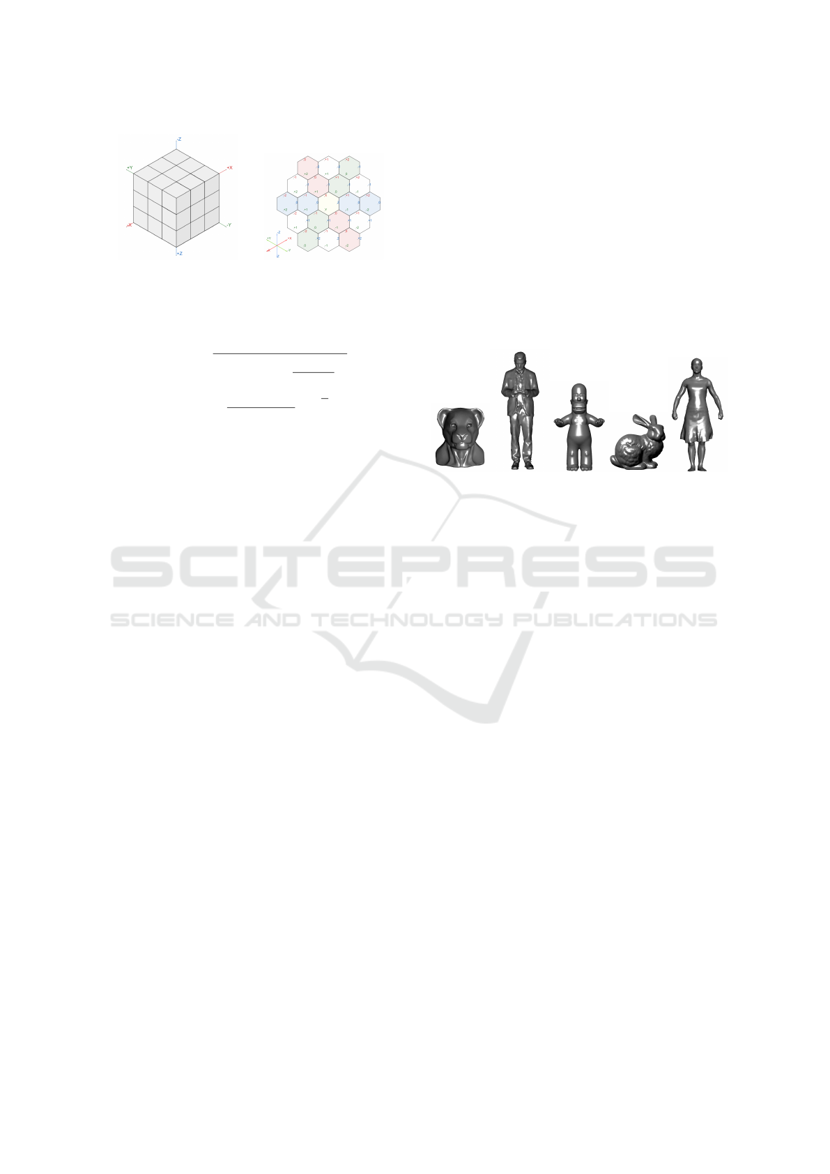
(a) Cube (b) Cube coordinates
for hexagonal grid
Figure 3: Cube coordinates for hexagonal grid.
centPeakDist:
triHeight =
r
(hexSize)
2
−(
hexSize
2
)
2
centPeakDist = (
2 ·triHeight
3
) ·
√
2.
The user also specifies the maximum number of lay-
ers to be generated (maxLayers).
The used approach for determining the closest
hexagon to the end point works as follows:
1. Get the default direction vector as~v = V
1
−V
0
2. Calculate centPeakDist
3. Calculate distance from the starting point to the
end point and save as d, set i = 1
4. Generate cube coordinates for hexagons in layer i
5. Generate hexagons in layer i. Use the cube coor-
dinates to get the distance of each hexagon from
the starting point (centre of the central hexagon)
• For each hexagon in the current layer, check if
its centre is closer to the end point than d, if it
is, update d
• If d < centPeakDist, return this hexagon as the
closest one. End.
6. Increment the angle of direction by 60/i
7. If i > maxLayers, return hexagon of distance d.
End.
8. Increment i and go to 4.
5 EVALUATION
The experiments to verify the functionality of the
algorithm were carried out on five different data
sets (meshes), each with five different hexagon sizes
and three different reference meshes. The results
were compared to the performance of a reference
implementation of the EdgeBreaker algorithm with
weighted parallelogram prediction (V
´
a
ˇ
sa and Brun-
nett, 2013).
See the input meshes in section 5.1. The dif-
ferent types of reference meshes will be presented
in the following sections. Five different hexagon
sizes were selected as hexSizeX = length/X , where
X ∈ {1,1.5,2,2.5,3} and length is the length of
the first edge of the first triangle of the input mesh
and hexSizeX is the distance between two adjacent
hexagons’ centres.
5.1 Input Meshes
Fig. 4 shows the input meshes (meshes to be encoded)
which were used for the experiments.
(a) Mesh 1:
Lion
(b) Mesh 2:
Person
(c) Mesh 3:
Homer
(d) Mesh 4:
Bunny
(e) Mesh 5:
Samba
Figure 4: Input meshes.
Note: This section contains charts showing the dis-
tribution of layer numbers and their occurrences. The
layers (denoted on the x axis) are sorted by their num-
ber in ascending order. The maximum layers allowed
to be generated for these experiments was 500. Only
those layers which appeared at least once are visible
in the chart.
For every encoded mesh, MSE was computed as
well as bits per vertex (bpv) of the hexagon layers
and index lists using arithmetic coding, see subsec-
tion 5.2. Experiments on the input meshes were per-
formed with unsuitable, good and very good reference
meshes.
By unsuitable reference, we mean such a mesh
whose surface is not very similar to the surface of the
input mesh. These reference meshes were acquired by
running ten iterations of HC Laplacian Smoothing on
the input meshes using the MeshLab software. Fig. 5
shows a typical result achieved by encoding the Lion
mesh using an unsuitable reference mesh.
Good reference meshes were acquired by running
two iterations of HC Laplacian Smoothing on the in-
put meshes using the MeshLab software. Fig. 6 shows
a typical results achieved by encoding the Person
mesh using a good reference mesh.
Very good reference meshes were acquired by
running one iteration of Isotropic Explicit Remesh-
ing on the input meshes using the MeshLab software.
Fig. 7 shows a typical results achieved by encoding
GRAPP 2022 - 17th International Conference on Computer Graphics Theory and Applications
274
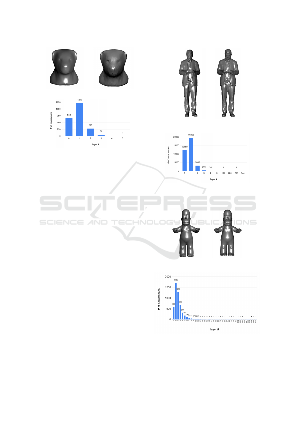
(a) Reference mesh (b) Decoded mesh
(c) Hexagon layers distribution
Figure 5: Lion mesh encoded using an unsuitable reference
mesh and hexSize2.
the Homer mesh using a very good reference mesh.
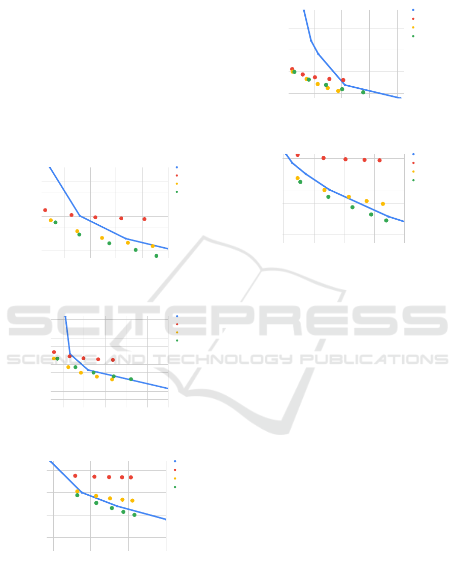
5.2 Mean Squared Error and BPV Data
This subsection contains information about the calcu-
lated MSE and bpv for each mesh. The data is shown
in Figures 8, 9, 10, 11 and 12. The results were
compared with the performance of the EdgeBreaker
algorithm with weighted parallelogram prediction.
The shown BPV is needed for encoding only the
geometry of the objects, the bitrate needed for en-
coding the connectivity is not taken into account, as
it is the same in both cases. The data shows that
our method is able to outperform the state of the art
algorithm, especially at very low bitrates, provided
that a good or very good reference mesh is available.
At higher bitrates, the proposed algorithm results in
a higher distortion, likely caused by projection on the
reference surface.
Although one could expect a more substantial im-
provement of coding efficiency, arguing that the shape
is actually known at the decoder, we believe that the
results in fact match a reasonable expectation. In-
tuitively, when a shape is fully unknown, there are
three degrees of freedom associated with each vertex.
When the shape is known and it is only the tessella-
tion that makes up the transmitted information, there
are still two degrees of freedom associated with each
vertex. If all degrees of freedom had the same statis-
tical properties, one could expect to save at most one
third of the data rate when a perfect shape reference
is available at the decoder.
(a) Reference
mesh
(b) Decoded
mesh
(c) Hexagon layers distribution
Figure 6: Person mesh encoded using a good reference
mesh and hexSize2.
(a) Reference
mesh
(b) Decoded
mesh
(c) Hexagon layers distribution
Figure 7: Homer mesh encoded using a very good reference
mesh and hexSize2.
Geometry Compression of Triangle Meshes using a Reference Shape
275
In practice, naturally, this assumption does not
hold. The tangential degrees of freedom may have
a different distribution than the original 3D coordi-
nates. On an abstract level, the key property is the ra-
tio of information entropy held by the tessellation (de-
pending on tessellation regularity in particular) and
the information entropy held by the shape itself (re-
lated mainly to the sampling density). It is for these
reasons that the practical results vary, as confirmed by
the presented experiments. Since the algorithm pro-
vides a performance improvement even when the ref-
erence mesh does not fully match the encoded shape,
we conclude that it works correctly.
BPV
MSE
0.001
0.005
0.01
0.05
0.1
4.0 4.5 5.0 5.5 6.0
Edgebreaker
Unsuitable
Good
Very Good
Figure 8: Performance comparison on the Lion mesh.
BPV
MSE
0
0.000001
0.000005
0.00001
0.00005
0.0001
0.0005
3.5 4.0 4.5 5.0 5.5 6.0
Edgebreaker
Unsuitable
Good
Very Good
Figure 9: Performance comparison on the Person mesh.
BPV
MSE
0.0001
0.001
0.01
0.1
4 6 8 10
Edgebreaker
Unsuitable
Good
Very Good
Figure 10: Performance comparison on the Homer mesh.
BPV
MSE
1.0E-07
1.0E-06
1.0E-05
1.0E-04
3.5 4.0 4.5 5.0
Edgebreaker
Unsuitable
Good
Very Good
Figure 11: Performance comparison on the Bunny mesh.
BPV
MSE
0.001
0.005
0.01
0.05
4 5 6 7 8
Edgebreaker
Unsuitable
Good
Very Good
Figure 12: Performance comparison on the Samba mesh.
6 CONCLUSIONS
We have presented a compression algorithm for tri-
angle meshes that uses a reference mesh of similar
shape to reduce the required data rate. Although the
reference shape undoubtedly provides quite a lot of
information about the input mesh, exploiting it turns
out to be a non-trivial task, since the particular choice
of sampling of the shape represents a major portion
of the data needed for defining a triangle mesh. The
results, however, demonstrate that our algorithm suc-
ceeds at this task using a novel combination of intrin-
sic encoding and hexagonal grid quantization.
In the current state, the algorithm is only practi-
cal for offline encoding, since the encoding is sub-
stantially slower than the decoding, because of the
exhaustive search for closest hexagon centre. This
does not eliminate all practical scenarios, because of-
ten meshes are indeed encoded offline and stored for
later processing, and the limiting factors are transmis-
sion time (which is improved due to better compres-
sion efficiency), and decoding time, which is much
faster than the encoding.
In the future, we would like to investigate a more
efficient means of finding the nearest hexagon centre.
We have already performed experiments with a vari-
ant of walking algorithm with promising results, more
tests are, however, still needed.
GRAPP 2022 - 17th International Conference on Computer Graphics Theory and Applications
276

Also, we would like to explore possibilities of bet-
ter mapping of local quantization areas to the curved
surface of the reference mesh. It is well known that
hyperbolic vertices, i.e. vertices with sum of inci-
dent angles larger than 2π, compromise the bijectivity
of the exponential map, creating a certain ”shadow”
which cannot be reached by walking along a straight
line. Overcoming this problem could lead to a further
reduction of the data rate.
Finally, in the future we would like to perform
experiments with an additional correction layer rec-
tifying the projection error and making it possible to
reach an arbitrary coding precision. We believe that
this way we could use our approach to obtain a data
rate advantage that propagates even to higher data
rates/lower reconstruction errors, since even the com-
peting algorithms are only able to predict the vertex
positions up to a certain precision, and additional pre-
cision is encoded at the cost/entropy of a fully random
data source.
ACKNOWLEDGEMENTS
This work was supported by the project 20-02154S
of the Czech Science Foundation. Eli
ˇ
ska Mourycov
´
a
was partially supported by the University specific re-
search project SGS-2019-016 Synthesis and Analysis
of Geometric and Computing Models. The authors
thank Diego Gadler from AXYZ Design, S.R.L. for
providing the test data.
REFERENCES
Alliez, P. and Desbrun, M. (2001). Valence-Driven Connec-
tivity Encoding for 3D Meshes. Computer Graphics
Forum.
Caillaud, F., Vidal, V., Dupont, F., and Lavou
´
e, G. (2016).
Progressive compression of arbitrary textured meshes.
Computer Graphics Forum, 35(7):475–484.
Chen, C., Xia, Q., Li, S., Qin, H., and Hao, A. (2018). High-
fidelity compression of dynamic meshes with fine
details using piece-wise manifold harmonic bases.
In Proceedings of Computer Graphics International
2018, CGI 2018, page 23–32, New York, NY, USA.
Association for Computing Machinery.
Corsini, M., Larabi, M. C., Lavou
´
e, G., Pet
ˇ
r
´
ık, O., V
´
a
ˇ
sa, L.,
and Wang, K. (2013). Perceptual Metrics for Static
and Dynamic Triangle Meshes. Computer Graphics
Forum.
Hoppe, H. (1996). Progressive meshes. In Proceedings
of the 23rd Annual Conference on Computer Graph-
ics and Interactive Techniques, SIGGRAPH ’96, page
99–108, New York, NY, USA. Association for Com-
puting Machinery.
Liang, K. K. (2018). Efficient conversion from rotating ma-
trix to rotation axis and angle by extending rodrigues’
formula.
Rossignac, J. (1999). Edgebreaker: Connectivity compres-
sion for triangle meshes. IEEE Transactions on Visu-
alization and Computer Graphics, 5(1):47–61.
Sorkine, O., Cohen-Or, D., and Toldeo, S. (2003). High-
pass quantization for mesh encoding. In Proc. of Euro-
graphics Symposium on Geometry Processing, pages
42–51, Aachen, Germany. Eurographics Association.
Touma, C. and Gotsman, C. (1998). Triangle mesh com-
pression. In Graphics Interface, pages 26–34.
Tutte, W. T. (1962). A census of planar triangulations.
Canadian Journal of Mathematics, 14:21–38.
V
´
a
ˇ
sa, L. and Brunnett, G. (2013). Exploiting connectiv-
ity to improve the tangential part of geometry predic-
tion. IEEE Transactions on Visualization and Com-
puter Graphics, 19:1467–1475.
V
´
a
ˇ
sa, L. and Dvo
ˇ
r
´
ak, J. (2018). Error Propagation Control
in Laplacian Mesh Compression. Computer Graphics
Forum.
Valette, S. and Prost, R. (2004). Wavelet-based progressive
compression scheme for triangle meshes: Wavemesh.
IEEE Trans. Vis. Comput. Graph., 10(2):123–129.
Geometry Compression of Triangle Meshes using a Reference Shape
277
