The Gopher Grounds: Testing the Link between Structure and Function

in Simple Machines

Anshul Kamath

1,† a

, Jiayi Zhao

2,† b

, Nick Grisanti

1 c

and George D. Monta

nez

1 d

AMISTAD Lab, Department of Computer Science, Harvey Mudd College, Claremont, CA, U.S.A.

Department of Computer Science, Pomona College, Claremont, CA, U.S.A.

Keywords:

Structure and Function, Agents, Genetic Algorithms.

Abstract:

Does structure dictate function and can function be reliably inferred from structure? Previous work has shown

that an artiﬁcial agent’s ability to detect function (e.g., lethality) from structure (e.g., the coherence of traps)

can confer measurable survival advantages. We explore the link between structure and function in simple

combinatorial machines, using genetic algorithms to generate traps with structure (coherence) and no function

(no lethality), generate traps with function and no structure, and generate traps with both structure and func-

tion. We explore the characteristics of the algorithmically generated traps, examine the genetic algorithms’

ability to produce structure, function, and their combination, and investigate what resources are needed for the

genetic algorithms to reliably succeed at these tasks. We ﬁnd that producing lethality (function) is easier than

producing coherence (structure) and that optimizing for one does not reliably produce the other.

1 INTRODUCTION

Recent research has shown that intention perception

(the ability to detect the intentions of others) can ben-

eﬁt artiﬁcial agents in a variety of adversarial situa-

tions (Maina-Kilaas et al., 2021a; Maina-Kilaas et al.,

2021b; Hom et al., 2021). One study found that when

artiﬁcial agents were able to perceive their environ-

ments as intentionally designed (e.g., to detect traps),

their survival rates signiﬁcantly increased (Hom et al.,

2021). Within their framework of virtual gophers and

projectile traps, Hom et al. assumed that traps de-

signed to harm gophers were much more likely to be

“coherent” than those generated uniformly at random,

and used this coherence as a basis for creating statis-

tical hypothesis tests (classifying traps as designed

to harm or unintended). Implicit within their ex-

perimental framework was an assumed correlation be-

tween the structure of a trap and its lethality: coher-

ence implied design which implied lethality. In this

study, we test whether the correlation between coher-

ence (structure) and lethality (function) was isolated

https://orcid.org/0000-0002-1641-4430

https://orcid.org/0000-0003-2497-120X

https://orcid.org/0000-0002-6987-9194

https://orcid.org/0000-0002-1333-4611

†

Denotes equal ﬁrst-authorship.

to their particular context, or whether the relationship

holds more generally.

The relationship between structure and function is

of general importance to science and engineering, as

every machine has structure that at least partially de-

termines its function. In Hom et al.’s work, coherence

(a property of trap structure) served as a reliable in-

dicator of trap functionality, able to separate human-

designed traps from those generated uniformly at ran-

dom. While Hom et al. considered only two types of

trap-generating processes, we explore the relationship

between trap coherence and trap functionality more

broadly, for machines generated by processes such as

genetic algorithms.

Genetic algorithms are an easy-to-implement

metaheuristic method commonly used to solve opti-

mization and search problems. They employ biolog-

ically inspired operators such as mutation, crossover

and selection (Golberg, 1989; Mitchell, 1998; Reeves

and Rowe, 2002). Genetic algorithms can solve prob-

lems deﬁned over complex, high-dimensional, multi-

modal, and/or discrete spaces. They have become a

popular optimization tool for structural optimization,

which is the automated synthesis of mechanical com-

ponents based on structural considerations (Chapman,

1994; Wang et al., 2006). Generating traps with

desirable traits, namely coherence and lethality, can

be considered as a simpliﬁed structural optimization

528

Kamath, A., Zhao, J., Grisanti, N. and Montañez, G.

The Gopher Grounds: Testing the Link between Structure and Function in Simple Machines.

DOI: 10.5220/0010900900003116

In Proceedings of the 14th International Conference on Agents and Artiﬁcial Intelligence (ICAART 2022) - Volume 2, pages 528-540

ISBN: 978-989-758-547-0; ISSN: 2184-433X

problem over a discrete search space, motivating their

use in the present study.

We examine the correlation between trap coher-

ence and trap lethality for structures produced by ge-

netic algorithms and ﬁnd that Hom et al.’s implicit as-

sumption may not hold in all situations. Furthermore,

we investigate genetic algorithms’ capacity to gener-

ate functional and coherent traps, given that humans

have little difﬁculty producing them. Finally, to the

extent our genetic algorithms are successful, we de-

termine what information resources are necessary for

them to generate traps with either lethality or coher-

ence (or both), by varying the information encoded in

their ﬁtness functions. We ﬁnd that contrary to asser-

tions by earlier researchers (e.g., (H

aggstr

om, 2007)),

simply having ﬁtness functions with structural order

(such as local neighborhood clustering) is not sufﬁ-

cient for genetic algorithms to perform the search task

any better than blind uniform sampling. To the con-

trary, we ﬁnd that alignment of the ﬁtness functions

to the particular task at hand is also necessary, agree-

ing with other prior work (Monta

nez, 2017; Monta

nez

et al., 2019).

2 RELATED WORK

There has been a wide range of research on the

relationship between structure and function. Gero

and Kannengiesser proposed the Function-Behaviour-

Structure ontology (Gero and Kannengiesser, 2007),

which provides three categories for the properties of a

human-designed object: Function (F), Behavior (B),

Structure (S). They assert that function (F) is “as-

cribed to” behaviour (B) by establishing a teleologi-

cal connection between a human’s design purpose and

what the object does, while behaviour (B) is “derived

from” structure (S) directly. Thus, they imply there is

no direct connection between function and structure.

Bock and Wahlert, however, argue that structure

and function constitute the two inseparable dimen-

sions of biological features when considering mor-

phology and evolutionary biology, and “must always

be considered together” (Bock and Wahlert, 1965).

Weibel proposed the theory of symmorphosis, which

predicts that the design of parts within an organism

must be matched to their functional demands. He also

tested these predictions by quantifying the relation-

ship between structure and function in different organ

systems (Weibel, 2000).

While Hom et al. only dealt with two kinds of

traps (those generated uniformly at random and those

they designed to be lethal (Hom et al., 2021)), we ex-

plore the lethality and coherence produced by a wider

variety of trap-generating processes. In particular, we

generate traps with structure (coherence) and no func-

tion (lacking lethality), traps with function and no

structure, and traps with both structure and function,

by means of genetic algorithms.

Genetic algorithms compose part of the larger

ﬁeld of evolutionary optimization (Golberg, 1989;

Mitchell, 1998; Reeves and Rowe, 2002). Evolu-

tionary optimization has been applied to a diverse

range of problems, with their associated difﬁculties.

One such difﬁculty is uncertainty—ﬁtness functions

are often noisy or approximated, environmental con-

ditions change dynamically, and optimal solutions

may change over time (Krink et al., 2004; Then and

Chong, 1994; Bhattacharya et al., 2014). A wide

range of techniques have been developed to combat

such problems (Jin and Branke, 2005).

3 METHODS

3.1 Traps

We adapt the virtual trap framework of Hom et al.

(Hom et al., 2021). A trap contains food to entice

an artiﬁcial gopher to enter and laser beams to “kill”

the gopher once it is inside. The traps are simple,

combinatorial objects embodying both form and func-

tion. This allows us to explore that relationship in a

controlled manner while investigating the effect of ge-

netic algorithm processes on their generation.

Each trap consists of a 4 ×3 grid. Three of the

tiles are ﬁxed for all traps: one acts as an entrance and

senses when the gopher enters the trap; directly above

the entrance is a ﬁxed blank ﬂoor tile that the gopher

can traverse to get to the third ﬁxed tile, which holds

the food enticing the gopher to enter the trap. The

remaining nine tiles can either be blank ﬂoor, laser

emitters (arrows), or wires meant to connect the laser

emitters to the sensor at the entrance. The arrows and

wires can be one of three thicknesses, with elements

of greater thickness more likely to kill a gopher. In

particular, the probabilities of killing a gopher on a

successful hit with a wide, normal, skinny arrow are

k,w

= 0.45, P

k,n

= 0.3, and P

k,s

= 0.15 respectively.

Two example traps are shown in Figure 1.

The laser will only be functional if the thickness

of the arrow matches the thickness of every wire piece

connecting it to the sensor. A wire tile can either be

straight or bent at a right angle, and can be rotated

by 90

◦

as needed. Arrows can similarly be rotated by

◦

. Accounting for all possible rotations and thick-

nesses, there are a total of 91 possibilities each of

these nine tiles can take. Hence—keeping in mind

The Gopher Grounds: Testing the Link between Structure and Function in Simple Machines

529

(a) Example of a func-

tional trap generated by

the genetic algorithm.

(b) Example of a designed

trap created by Hom et al.

Figure 1: Example traps.

that the entrance and food tiles are each used exactly

once per trap—there is a total of 91

≈ 4.28 ×10

possible traps in this framework. We let X denote the

set of all valid traps, with |X | ≈ 4.28 ×10

In agreement with Hom et al., we deﬁne trap co-

herence as follows (Hom et al., 2021). First, we must

deﬁne the notion of a coherent connection. There is a

coherent connection between two non-entrance tiles if

all of the following conditions are met: (1) both tiles

contain either a wire or an arrow, (2) the thicknesses

of the two elements match, and (3) the two elements

share an endpoint (i.e., the rotation of the wires align).

The coherence of a trap is then the number of coher-

ent connections per nonempty (wire or arrow) tiles.

Furthermore, we deﬁne the lethality of a trap as

the probability that it kills a gopher entering it. Also

referred to as functionality in this context, lethality

can either be estimated by running simulations that

present traps to gophers of varying hunger levels and

measure the proportion of gophers killed, or com-

puted analytically. We compute both coherence and

functionality analytically, with empirical simulation

verifying the correctness of our approach (not shown).

3.1.1 Trap Encoding

We introduce a genotypic representation of a trap

(called an encoding) for our genetic algorithm. Our

encoding method takes in a 4 ×3 trap matrix and out-

puts a 1×12 array of integers. First, we look at the 93

individual tiles and map each of them to a unique in-

teger x ∈ [0,92]. For instance, the skinny arrow with

right-acute angle rotated at 0

◦

has the encoding 33.

Note that the encoding for door tile is 0, food tile 1,

and the ﬂoor tile 2. The encoding for each tile of an

example trap is shown in Figure 2a.

(a) Encodings for 12 trap

tiles.

(b) Indexing the 12 trap

tiles.

Figure 2: Tile encoding and trap location indexing.

Next, we enumerate the 12 tiles in a trap as

shown in Figure 2b. Intuitively, each trap can be en-

coded by listing the encodings of its tiles in the order

(0,1, 2, 3,4,5, 6, 7,8, 9, 10,11), creating a zig-zag pat-

tern; this is Method 1, demonstrated in Figure 3. A

potential problem with this method is that the order

of the tiles in an encoding does not reﬂect the spatial

layout of the trap. See, for example, how tiles 2 and

3 are positioned on opposite sides of the trap but are

ordered sequentially in the encoding. To address this,

we developed an additional method, Method 2, which

encodes a trap by listing the encodings of its tiles in

the order (9, 6,3, 0, 1,2, 5, 8,11, 10, 7,4). This order

lists the traps in a wrap-around pattern, as shown in

Figure 4. Thus, sequential tile encodings in the trap

encoding are adjacent to each other in the actual trap.

3.2 Gophers

Like Hom et al., we used gophers as the artiﬁcial

agents in our experiments. Hom et al. designed

two types of gophers: intention gophers and base-

line gophers. Intention gophers were given inten-

tion perception—the ability to assess the coherence

of the trap and then determine if the trap is deliber-

ately harmful, based on its coherence. If the trap is

found sufﬁciently coherent, the intention gopher will

avoid it; otherwise, the gopher will enter it. Base-

line gophers, however, will enter any trap according

to some predetermined probability. Whereas Hom et

al. compared survival outcomes of intention and base-

line gophers, we seek to merely assess the coherence

and lethality of traps generated using a genetic algo-

rithm. As such, we simplify our gopher framework to

ICAART 2022 - 14th International Conference on Agents and Artiﬁcial Intelligence

530

(a) Encoding with permu-

tation (0, 1, 2, 3, 4, 5, 6, 7,

8, 9, 10, 11)

(b) Encoded trap: [47, 6,

86, 25, 1, 29, 26, 2, 62, 72,

0, 9]

Figure 3: First encoding method and corresponding en-

coded trap, Method 1.

(a) Encoding with permu-

tation (9, 6, 3, 0, 1, 2, 5, 8,

11, 10, 7, 4)

(b) Encoded trap: [72, 26,

25, 47, 6, 86, 29, 62, 9, 0,

2, 1]

Figure 4: Second encoding method and corresponding en-

coded trap, Method 2.

include only one type of gopher, which is described

below. Each gopher has a hunger level H uniformly

sampled from {0,0.2,0.4, 0.6,0.8}, and will enter a

trap with probability

(H) = P

·(1 −H

) + H

where P

is the default probability of entering (what

a baseline gopher would have in Hom et al.’s frame-

work) and H ∈ [0, 1) is the current hunger level.

The eating time t

eat

of the gopher is how long (in

discrete time steps called frames) the gopher takes to

eat and is selected according to the probability vector

~p = [p

, p

where, p

is the probability that a gopher eats for j

frames. By this deﬁnition of ~p, each gopher will take

between 1 and 5 frames (inclusive) to eat. The prob-

ability vector ~p depends only on the default probabil-

ity of entering P

, and it is calculated by methods in

(Hom et al., 2021).

When a gopher decides to enter a trap, it will di-

rectly head to the food with speed 1 tile/frame, eat for

eat

frames, and then exit the way it came with speed

1 tile/frame. When the gopher ﬁrst enters the trap,

the sensor will detect it instantly and release a pulse

on each side of the entrance door. If the arrow is co-

herently connected to the door, the pulse will travel

through the wire with speed 1 tile/frame and ﬁre a

projectile with speed 1 tile/frame that can possibly hit

the gopher. We designed our gophers to be “skittish,”

that is, they ﬂee traps whenever a laser ﬁres, regard-

less of their hunger level.

3.3 Genetic Algorithms

In mimicking natural selection, genetic algorithms

optimize toward increasing ﬁtness. Here the popu-

lation consists not of biological organisms but of po-

tential solutions to an optimization problem.

A genetic algorithm requires a ﬁtness function

(see below) to generate a subset of elements X ⊆ X .

In our setting, for example, X is the set of all valid

traps deﬁned in Section 3.1. Then, the algorithm

goes through a process of selection, recombination,

and mutation to generate a new subset X

⊆ X . The

algorithm usually begins with a generation of ran-

domly generated elements. For each generation of

the genetic algorithm, a subset of the population is

selected to “reproduce” to ﬁll the next generation’s

population. Much as organisms of higher ﬁtness in

nature are more likely to reproduce (by deﬁnition),

elements of higher ﬁtness in the genetic algorithm are

more likely to contribute to the next generation. To

achieve this, we used a roulette-wheel selection pro-

cess: two elements of the previous generation are se-

lected at random, with their probability of selection

directly proportional to their ﬁtnesses. These two

elements undergo a recombination process in which

their information is combined—usually by splicing

each element in two and sampling a piece from each

element—to produce a new element that contains in-

formation from both parents. Example of such splits

are shown in Figure 5.

Finally, we mutate the resulting element by ﬂip-

ping a random element in its encoding to some ran-

dom value in the cell alphabet, in the style of a genetic

point mutation. This element is now fully formed and

joins the new generation. The process repeats until the

size of the new generation matches that of the old gen-

The Gopher Grounds: Testing the Link between Structure and Function in Simple Machines

531

(a) Method 1 (b) Method 2

Figure 5: An example of recombining at the ﬁfth cell under

both encoding methods.

eration. New generations are iteratively created until

some threshold is met, usually requiring that one of

the elements have a ﬁtness above a speciﬁed value or

that a speciﬁc number of generations is produced. The

single element with highest ﬁtness is then returned.

Algorithm 1 provides pseudocode for this entire pro-

cess, where f (·) is the ﬁtness evaluation function.

Algorithm 1: Sample Genetic Algorithm.

1: procedure GENETICALGORITHM

2: globalBest ← none

3: population ← generateRandomPopulation()

4: while not terminationConditionsMet do

5: newPopulation ← empty

6: for element in population do

7: selectedPair ← roulette(population)

8: combined ←recombine(selectedPair)

9: mutated ← pointMutate(combined)

10: newPopulation.add(mutated)

11: popBest ← bestTrap(newPopulation)

12: if f (popBest) > f (globalBest) then

13: globalBest ← popBest

14: population ← newPopulation

15: return globalBest

3.4 Fitness Functions

To determine the optimality of a member x ∈ X , we

deﬁne a ﬁtness function. This function f : X → R

allows us to impose an ordering on the elements of

the search space, X , thereby giving the algorithm a

measure of how optimal the current solution is. We

next describe our process for creating a set of ﬁtness

functions based on different optimization criteria. To

make our language more precise, we deﬁne the order

and alignment of a ﬁtness function. Order within a

ﬁtness function refers to any underlying patterns or

regularities that may be present in its spatial distribu-

tion of values, such as local neighborhood clustering.

The alignment of a ﬁtness function refers to the mea-

sure of preference for elements in a speciﬁc target set

of interest. For example, if we want to optimize for

coherence, a ﬁtness function is correctly aligned if it

gives high ﬁtness values to coherent traps and low ﬁt-

ness values to non-coherent traps.

In the subsections that follow, we describe the ﬁt-

ness functions used in our experiments.

3.4.1 Random Fitness

For any trap x ∈X , we deﬁne the random ﬁtness func-

tion as r(x) = n where n is a number chosen uniformly

at random from the range [0,1). In other words, when

running the genetic algorithm, we impose a random

ordering on the population through the random ﬁtness

function and select traps according to this random or-

dering. Thus, we do not expect the random ﬁtness

function to exhibit either order or alignment.

3.4.2 Binary Distance (Hamming) Fitness

Let t ∈X be a uniformly sampled random trap, and let

it serve as our target trap. The binary distance ﬁtness

function returns a number indicating how “close” a

given trap to the target trap t.

For any trap x ∈ X , we deﬁne the binary distance

ﬁtness to be

d(x) =

diff

total

where #

diff

is the number of differences in the tiles

between x and t, and #

total

is the maximum number

possible differences; this value is 12 −3 = 9 as, it ex-

cludes the three ﬁxed cells—door, ﬂoor, and food—

in the middle column of every trap. Thus, this ﬁtness

function will quantify how close x is to t, thereby giv-

ing it local neighborhood structure and order. How-

ever, this measure does not give us any meaningful in-

formation about the coherence or lethality of the trap.

Hence, this ﬁtness function is not aligned.

3.4.3 Functional Fitness (Lethality)

For any trap x ∈X , we deﬁne the functional ﬁtness by

f (x) =

kill

(x)

max

which is the normalized probability that the trap x will

kill the gopher. P

kill

(x) is the (non-normalized) prob-

ability that the trap x will kill the entering gopher, and

max

is the maximum probability of a gopher dying.

ICAART 2022 - 14th International Conference on Agents and Artiﬁcial Intelligence

532

We calculate these values analytically (as detailed in

Appendix A).

Our ﬁtness function f (x) evaluates the functional-

ity of traps in terms of killing gophers. Since it gives

higher values to lethal traps and similar traps often

have similar lethality, this ﬁtness function has both

order and alignment.

3.4.4 Coherent Fitness

Following Hom et al., for any trap x ∈ X , we deﬁne

the coherent ﬁtness function as

g(x) =

where c

is the total number of coherent connections

and t

is the number of nonempty cells (Hom et al.,

2021). Since g(x) gives higher values to coherent

traps and similar traps have similar coherence, this ﬁt-

ness function has both alignment and order, as well.

3.4.5 Multiobjective Fitness

For clariﬁcation, we will deﬁne two different ﬁtness

functions in this section. Both of them aim to priori-

tize traps that are both lethal and coherent, penalizing

large gaps between coherence and lethality values (so

that the process does not merely optimize for lethality

at the expense of coherence, for example).

We deﬁne a global multiobjective ﬁtness function

h : X → R which takes a trap as an input and out-

puts a ﬁtness value representing both coherence and

lethality of the trap. This ﬁtness function is similar

to functional and coherence ﬁtness functions, but it

is not efﬁcient enough when optimizing multiple ob-

jectives. Therefore, we implement an additional local

multiobjective ﬁtness function, ϕ : X

→ R

, where

n ∈ N is the population size. The function takes in

a population of traps and outputs a ﬁtness value for

each, effectively imposing a partial ordering on the

current population. The local multiobjective ﬁtness

function only provides relative ranks of traps within

a generation; the same trap can be assigned different

ﬁtness values in different generations, making it dif-

ﬁcult to compare traps across generations, which was

necessary for our analysis.

Therefore, we use the global multiobjective ﬁtness

value of each trap for record-keeping and analysis,

and use the local multiobjective ﬁtness function for

selection within the genetic algorithm, for efﬁciency.

We describe both ﬁtness functions in detail next.

Local Multiobjective Fitness. We begin by deﬁn-

ing a notion of dominance among traps. Trap A dom-

inates trap B if trap A has both a greater functional

ﬁtness and a greater coherent ﬁtness than trap B.

Our local multiobjective ﬁtness function is deﬁned

as follows. Each trap in the population is given a base

score, which is equal to one more than the number of

traps it dominates. Next, to disincentivize sampling

traps that are too similar to each other, we compute the

point-wise Euclidean distance between each trap and

its closest neighbor of the same base score. If there

is only one trap of a particular base score, then the

distance is deﬁned to be

√

2 (the maximum possible

distance between two traps). The point-wise distance

for each trap is divided by

√

2 and added to its base

score to determine its boosted score. Each boosted

score is then divided by the maximum boosted score

across the population, leaving the most ﬁt trap with a

ﬁtness value of 1. This set of boosted scores—which

is contained in the interval (0,1]—is then returned.

This function is a variation of a standard method

for multiobjective evolutionary optimization (Fonseca

et al., 1993). The number of other traps a particular

trap dominates is a good measure of overall ﬁtness,

as traps with either a greater functional or coherent

ﬁtness are likely to dominate more traps. By boost-

ing each trap’s score by an amount proportional to its

distance from the nearest neighbor of the same base

score, the genetic algorithm is disincentivized from

sampling traps that are too similar to each other. This

should not only help the genetic algorithm reach a ﬁt-

ness threshold more quickly, but encourage popula-

tions to become diverse.

Global Multiobjective Fitness. For any trap x ∈X ,

we deﬁne the global multiobjective ﬁtness to be

(x) =

f (x) + g(x)

2|f (x)−g(x)|

where f (x) and g(x) are the functional and coherent

ﬁtness values of x, respectively. We sought to mini-

mize the difference between f (x) and g(x) in the ﬁnal

generated trap, so we introduced another penalty to

disincentivize solely optimizing coherence or lethal-

ity alone (which could lead to large gaps between the

functional and coherent ﬁtness values):

h(x) =

(

(x) |f (x) −g(x)| ≤ k

di f f

10k

di f f

(x) |f (x) −g(x)| > k

di f f

where k

di f f

is some constant we deﬁned. Further-

more, since this ﬁtness function assigns higher values

to traps that are both lethal and coherent, it also has

both order and alignment.

4 EXPERIMENTAL SETUP

The general framework for our experiments consists

of generating a trap using our genetic algorithm, then

The Gopher Grounds: Testing the Link between Structure and Function in Simple Machines

533

assessing the trap to determine what expected propor-

tion of gophers would die when entering it.

To generate a single satisfactory trap—a trap opti-

mized for either random ﬁtness, hamming ﬁtness, co-

herence ﬁtness, functional ﬁtness, or multiobjective

ﬁtness—we create an initial population of size 20 and

run the genetic algorithm with its corresponding ﬁt-

ness function for 10,000 generations. Then, we out-

put the trap with the highest ﬁtness value among all

200,000 traps. We repeated this process 1,000 times

for each ﬁtness function, performing 1,000 indepen-

dent trials and thus generating 1,000 optimized traps

for each.

Additionally, in order to compare our experiments

to some baseline distribution, we randomly generate

the same number of traps uniformly at random. We

also use the designed trap’s given by Hom et al. as

a control for highly coherent and lethal traps (Hom

et al., 2021).

5 RESULTS

5.1 Proportion Vectors

First, we show the coherence and lethality distribu-

tions of traps generated by genetic algorithms with

different ﬁtness functions. Figure 6 depicts the pro-

portion of traps at given lethality/coherence levels,

separated by each method used to generate the traps.

Analyzing these vectors, we notice that the ran-

dom, uniform, and binary distance methods give iden-

tical proportion vectors with respect to both lethal-

ity and coherence. This suggests two things; ﬁrst,

that uniform random sampling of traps is as effec-

tive as using a genetic algorithm equipped with a ﬁt-

ness function that randomly assigns each trap its ﬁt-

ness value. Second, it suggests that simply having or-

der in a ﬁtness function is not sufﬁcient to improve

the probability of success (contrary to (H

aggstr

om,

2007)): ﬁtness functions must also have intentional

alignment, which leads the genetic algorithm towards

a target set of interest. Since the binary distance ﬁt-

ness function chooses a random target trap and tries

to generate similar traps, we can see that this ﬁtness

function has sufﬁcient order, but it does not align

with the problem of optimizing for coherence and/or

lethality. In other words, genetic algorithms with ran-

dom, uniform random, and binary distance ﬁtness

functions only perform as well as uniform random

sampling in terms of generating coherent and/or lethal

traps, due to their lack of correct alignment. More

simply, we must embed some selection bias towards

the target set into our ﬁtness function to get improved

results. It is not sufﬁcient to simply have order.

Next, note that the lethality ﬁtness function is not

aligned with the coherence ﬁtness function and vice

versa. More speciﬁcally, the coherence proportion

vector in Fig. 6a is highly similar to the uniform ran-

dom proportion vector when we optimize for lethality.

This is due to a mismatch in alignment. The intersec-

tion of the coherence and lethality target sets is too

small, so when we optimize for coherent traps, we do

not necessarily get lethal traps as well. The same rea-

soning explains why the lethality proportion vector in

Fig. 6b is highly similar to the uniform random pro-

portion vector when we optimize for coherence.

Moreover, notice that a large proportion of traps

reached maximum lethality in both the functional and

multiobjective experiments in Fig. 6a. While this

makes sense (since these ﬁtness functions were meant

to optimize for lethality), notice the same cannot be

said for coherence in Fig. 6b, whose maximum value

(of sufﬁcient magnitude such that it does not appear

white on the color bar) is 0.556. Thus, in 10,000

generations we have seen that at least ∼40% of traps

had maximum lethality when optimizing for lethal-

ity, while only ∼10% of traps had coherence of 0.556

when optimizing for coherence. This discrepancy

suggests that it is much easier to create lethal traps

than it is to create coherent traps. It is important to

note that the proportion of traps varies greatly. While

it appears there are no traps with coherence greater

than 0.556, there are, but not in signiﬁcant enough

quantities to show up in Figure 6b.

Additionally, notice that for uniform-random sam-

pling, there were traps sampled with lethality 0.215,

0.430, and 0.645. These all correspond to simple,

functional traps such as those shown in Figure 7.

Finally, we can notice that the human designed

traps of Hom et al. are starkly different from any traps

generated by our programs. Their traps were created

to simply zap gophers in a broad variety of ways; they

were not intentionally optimized for coherence nor for

perfect lethality, but optimized for diverse functional-

ity. However, we see that every designed trap had a

coherence of 1, and its lethality was essentially ran-

domly distributed. Thus, we can conﬁrm that the form

of a trap is a good indicator of intended construction.

It is also important to note that, as far as we are aware,

the human-designed traps of Hom et al. were not in-

tentionally designed to be highly coherent. Instead,

they were made to test all types of traps, as shown

by the uniform probability distribution for lethality in

Figure 6a. This unintended coherence could simply

be attributed to the fact that humans have an innate

sense of structure. However, this afﬁnity for structure

ICAART 2022 - 14th International Conference on Agents and Artiﬁcial Intelligence

534

(a) Lethality. (b) Coherence.

Figure 6: Heat map showing the proportion of traps with a given lethality / coherence, split by the parameter which the genetic

algorithm was optimizing for (and designed traps).

Figure 7: Four simple traps of lethality 0, 0.215, 0.430, and 0.645, respectively.

is challenging to imitate in silico, as shown by the

lack of coherent traps generated by our algorithms,

even when trying to optimize for coherence directly.

5.2 Time to Optimal Trap

Figure 8 shows when an optimal trap was found for

each trial. The functional ﬁtness function seems to

ﬁnd its optimal trap in roughly 100 generations. This

makes sense, since we have already seen that it is not

very hard to get a maximally lethal trap; all that is

needed are two angled, thick arrows on either side of

the door. Additionally, its interquartile range is ex-

tremely small (as shown by the outliers proximity to

the box) which provides further evidence of the ease

of ﬁnding a maximally lethal trap.

The coherence and multiobjective ﬁtness func-

tions are more interesting. They both have similar

(essentially the same) distributions, with medians at

roughly 3,000 generations (where the coherence dis-

tribution is slightly higher), and ranges spanning the

whole x-axis. The interquartile range is higher for the

multiobjective function.

Figure 9a shows the average optimal ﬁtness across

all generations. This is calculated as follows: take a

generation i in all 10,000 generations. We then take

the best observed ﬁtness up to generation i for each

trial, and then average them across all 1,000 trials.

This gives us monotonically increasing averages for

all three functions. For the functional ﬁtness function,

we notice that the curve approximates a step function.

This makes sense, since we know that the functional

experiments quickly converge to 1.0. The lack in vis-

ibility of the conﬁdence intervals is due to low vari-

ance in the outcomes. Notice, however, that the co-

herence and multiobjective curves converge at a much

slower rate. This is due to the increased difﬁculty in

ﬁnding coherence. Additionally, we note that these

values seem to approach roughly 0.75 and 0.6 respec-

tively, which indicate that these are the highest ﬁtness

values we found (on average). Finally, notice how the

change in the slope drastically falls off after genera-

tion 4,000. This is due to the fact that most of the

experiments have converged, and there are few traps

with higher ﬁtness left for the algorithm to ﬁnd.

On the other hand, Figure 9b shows the average

population ﬁtness across trials at a given generation,

The Gopher Grounds: Testing the Link between Structure and Function in Simple Machines

535

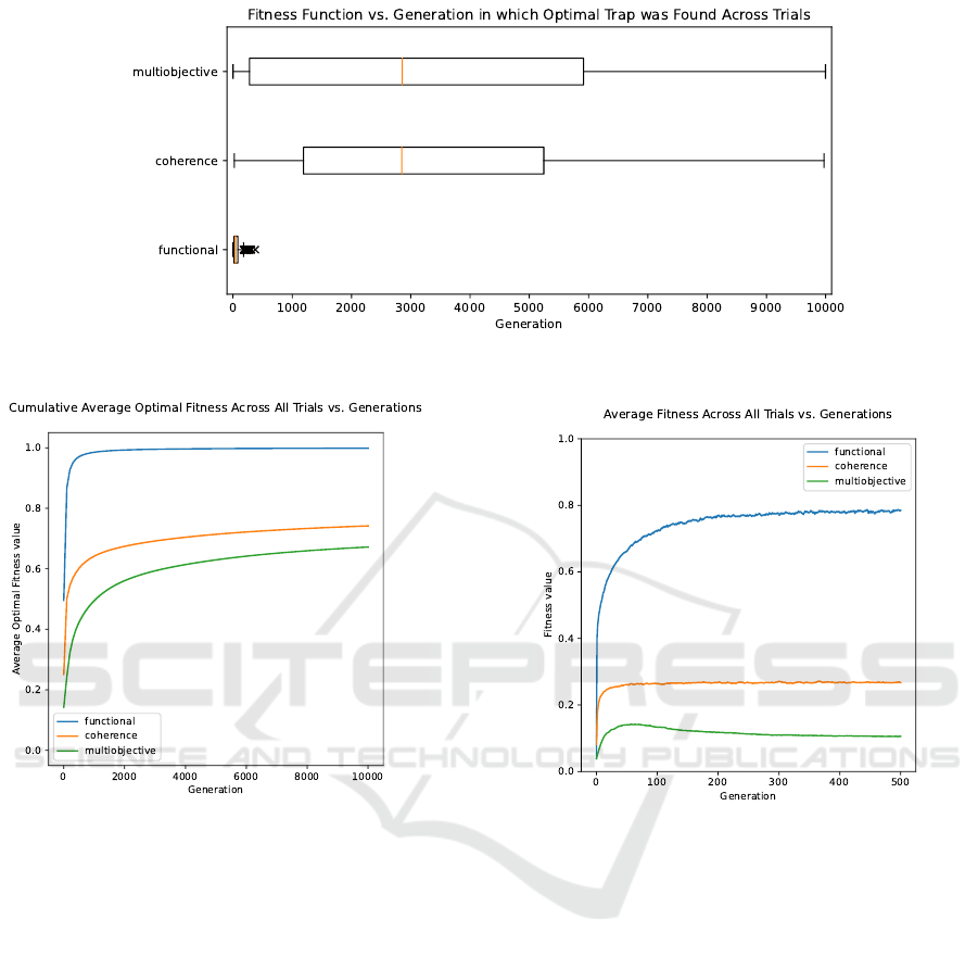
Figure 8: Boxplot showing the distribution of when the optimal trap was found across all generations.

(a) Line plot showing the cumulative average optimal ﬁt-

ness across all trials over generations. The shaded region

represents the 95% conﬁdence interval.

(b) Line plot showing the average ﬁtness across all tri-

als over generations. The (imperceptible) shaded region

again represents the 95% conﬁdence interval.

Figure 9: Line plots showing the trends of average ﬁtness over generations

for all generations. Unlike the previous graph, this

was made by taking a given generation of the algo-

rithm and averaging all the ﬁtnesses across the 1,000

trials (instead of the optimal cumulative ﬁtness). We

only plot generations 0-500 since there are no notable

deviations from the observed trend. As we can see,

the average ﬁtness across all trials seems to plateau

for each ﬁtness function. While this makes sense for

the functional ﬁtness function (since it arrives at its

max value the fastest), we notice that the average ﬁt-

ness for coherence and multiobjective plateau at com-

paratively low ﬁtness values of 0.25 and 0.1 respec-

tively. This is surprising, since our genetic algorithm

is equipped to generate coherent structures; we ex-

pected the average ﬁtness across generations to gen-

erally increase in the absence of ﬁnding the optimal

solution.

Finally, notice that there is a peak in the multiob-

jective curve. We believe this is due to the algorithm

ceasing to optimize for primarily lethal traps and in-

stead optimize for coherently lethal traps. In this

event, the algorithm would have to sacriﬁce lethality

in favor of coherence and lethality, which decreases

the overall ﬁtness.

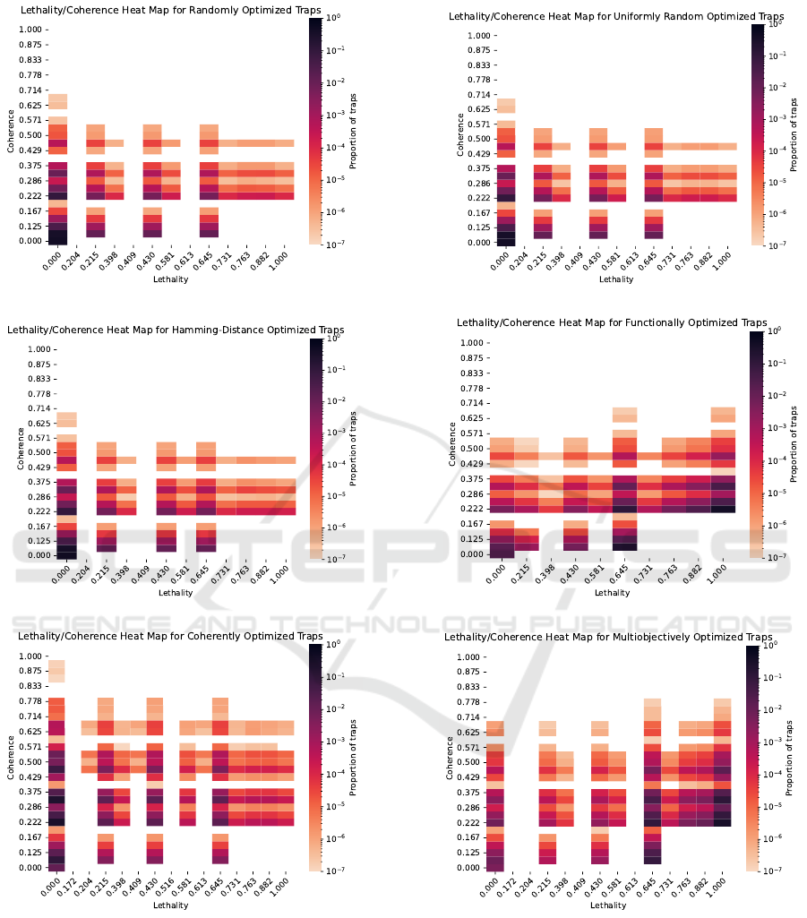
5.3 Frequency Density Heatmaps

Figures 10a - 10c show the log proportion of traps

with a given lethality and coherence value. Note that

all traps generated across the 10,000 generations of

the genetic algorithm are included in this dataset.

We can observe some shared trends in these

heatmaps; ﬁrst, notice that the most common lethality

values are 0, 0.215, 0.430, and 0.645. These all corre-

ICAART 2022 - 14th International Conference on Agents and Artiﬁcial Intelligence

536

(a) Random. (b) Uniform-random.

(e) Coherence. (f) Multiobjective.

Figure 10: Heatmaps representing the log proportion of traps with a given lethality and coherence value separated by opti-

mization parameter.

spond to simple, functional traps such as the examples

given in Figure 7.

Since these traps are quite simple, we observe that

it is not too difﬁcult for the algorithm to generate

lethal traps. To see this more clearly, consider the

coherence values below 0.222 (which corresponds to

having at most one coherent connection) among all

graphs. As is evident, there are only four possible

lethality values among these coherences, since any

coherence value below 0.222 indicates there is at most

The Gopher Grounds: Testing the Link between Structure and Function in Simple Machines

537

one functional arrow. Thus, we can see that lethal

traps also provide a baseline coherence, since the only

way a trap can be lethal is if it is built upon coherent

connections. An absolute lack of coherence implies a

lack of functionality.

Studying Figures 10a - 10c more closely, we can

see that these heatmaps look roughly the same. Thus,

this supports the idea that the random ﬁtness func-

tion, uniform-random sampling, and the binary dis-

tance function all generate results of similar quality

(as evidenced by the way they sample the same space

during the genetic algorithm process). More speciﬁ-

cally, the random and binary distance functions seem

to be as good as uniform random sampling, and they

cannot reliably produce coherent or lethal traps.

Finally, studying Figures 10d - 10f, we see that

the multiobjective heatmap shares characteristics with

both the functional and coherent heatmaps. More

speciﬁcally, we see that the multiobjective heat map

resembles the functional heatmap closely, except that

it shifts some frequency mass towards higher coher-

ence traps. This is evidence that the multiobjective

heatmap was successfully creating coherent and func-

tional traps, however it does not seem to be able to

reliably create highly functional and coherent traps.

6 DISCUSSION

We can see how the complexity of generating co-

herent traps factored into the multiobjective function.

While the multiobjective frequencies in Figure 10f re-

semble aspects of both the lethality and coherence fre-

quency plots, it is much further skewed towards the

lethality frequency plot. This is due to the fact that

our genetic algorithm could much more easily opti-

mize for lethality than coherence. We generally see

highly lethal traps within 200 generations. Observing

these lethality-optimized traps, it is apparent that the

genetic algorithm almost always produces traps with

the simplest form of lethality: arrows attached to the

side of the door. For these traps, a baseline level of co-

herence is guaranteed as they have two coherent con-

nections to the door. However, it is difﬁcult to gener-

ate traps with just these two arrows. Instead, most of

these functional traps have additional, non-functional

tiles that decrease their coherence.

While lethality-optimized traps usually reach

maximum lethality within 200 generations, the

coherence-optimized traps do not reach their maxi-

mum until ∼2,500 generations. We can attribute this

difference to the lack of a short-cut to coherence;

while we can generate extremely simple but func-

tional traps by attaching arrows to the door, coherent

traps by nature require coordination.

This may also suggest that there are more func-

tional traps than coherent traps. We can verify

this through simple calculations and sampling exper-

iments. Among all possible traps, there are at least

≈ 2.288 ×10

traps with lethality 1, even if we

only consider traps with two wide arrows directly at-

tached to the door, pointing at the middle column.

However, there are only 26,733 traps with coherence

1. Moreover, according our sampling of one mil-

lion uniform random traps, 2.27% of the traps have

lethality values greater than or equal to 0.5, but only

0.0037% of the traps have coherence values greater to

equal to 0.5.

Also note that the coherence of a trap is solely de-

termined by the connectedness of the wires, which

is a property that is not preserved under mutation

and recombination. On the other hand, many traps

can have arrows in the ﬁrst cell adjacent to the door,

so mutations and recombinations do not affect these

traps as much. Hence, as single, stepwise changes

may reduce, rather than improve ﬁtness, improve-

ments in trap coherence may require multiple, coor-

dinated changes in trap cells. Therefore, modifying

the genetic algorithm to allow coordinated mutations

and recombination may be a possible method to over-

come the current barriers to achieving high coherence

levels.

7 CONCLUSIONS

How strong is the link between coherence and lethal-

ity, representing structure and function? Since lethal

traps require at least one coherent connection, where

there is a lack of coherence, there is a correspond-

ing lack of lethality. However, it’s important to note

that even though high lethality guarantees a base-

line coherence (≥ 0.222) when producing lethality-

optimized traps, the genetic algorithm does not gen-

erate high coherence as a side-product. Similarly,

coherence alone does not beget lethality, but it may

boost the probability of ﬁnding ﬁring traps. So the

relationship, while present, is weak.

As we can see in Figure 6b, the designed traps

all have a coherence of 1, whereas the genetic al-

gorithm was not able to reliably achieve coherence

levels above 0.556 when optimizing for coherence.

These ﬁndings suggest that contingent coherence re-

mains a plausible sign of intentional construction, as

optimizing trap coherence is effortless for human de-

signers. This supports Hom et al.’s use of trap co-

herence as an indicator of intentional design in their

original experiment.

ICAART 2022 - 14th International Conference on Agents and Artiﬁcial Intelligence

538

Our genetic algorithms were able to generate cer-

tain types of traps well. Speciﬁcally, they were ef-

ﬁcient in generating highly functional traps, produc-

ing maximally lethal traps in a reasonably small num-

ber of generations. Coherent traps, however, were

much more difﬁcult to produce. The genetic algo-

rithms struggled to produce traps with high levels of

coherence, even when optimizing for coherence di-

rectly. Optimizing for both lethality and coherence

proved even more difﬁcult. Most of the traps gener-

ated had high lethality but relatively low coherence.

To reliably generate traps with high coherence

and/or lethality using genetic algorithms, both order

and correct alignment of ﬁtness functions were es-

sential. First, our ﬁtness functions required order,

with neighborhood constraints on the elements of the

search space, allowing a genetic algorithm to perform

a meaningful local search. However, order in the ﬁt-

ness functions was not enough, as was evident in the

failure of the binary distance ﬁtness function. To gen-

erate traps with speciﬁc characteristics (e.g., coher-

ence), the ﬁtness functions also needed to be correctly

aligned with a speciﬁc target set. In other words, op-

timizing for lethality did not reliably produce coher-

ence, and vice versa. Only when we designed a ﬁtness

function that was intelligently aligned to a speciﬁc

goal was the genetic algorithm able to successfully

produce traps with either the structural or functional

characteristics sought.

ACKNOWLEDGEMENTS

The authors would like to thank Cynthia Hom and

Amani Kilaas-Mainas for providing access to their

code and helpfully answering questions, and Tim

Buchheim for assistance in experimental set-up. This

research was supported in part by the National Sci-

ence Foundation under Grant No. 1950885. Any

opinions, ﬁndings, or conclusions expressed are the

authors’ alone, and do not necessarily reﬂect the

views of the National Science Foundation.

REFERENCES

Bhattacharya, M., Islam, R., and Mahmood, A. N. (2014).

Uncertainty and Evolutionary Optimization: A Novel

Approach. In 2014 9th IEEE Conference on Industrial

Electronics and Applications, pages 988–993.

Bock, W. J. and Wahlert, G. V. (1965). Adaptation and the

form–function complex. Evolution, 19.

Chapman, C. D. (1994). Structural Topology Optimization

via the Genetic Algorithm. PhD thesis, Massachusetts

Institute of Technology.

Fonseca, C. M., Fleming, P. J., et al. (1993). Genetic Algo-

rithms for Multiobjective Optimization: Formulation

Discussion and Generalization. In ICGA, volume 93,

pages 416–423.

Gero, J. S. and Kannengiesser, U. (2007). A Func-

tion–Behavior–Structure Ontology of Processes. Ar-

tiﬁcial Intelligence for Engineering Design, Analysis

and Manufacturing, 21(4):379–391.

Golberg, D. E. (1989). Genetic Algorithms in Search, Opti-

mization, and Machine Learning. Addison-Wesley.

aggstr

om, O. (2007). Intelligent design and the NFL the-

orems. Biology & Philosophy, 22(2):217–230.

Hom, C., Maina-Kilaas, A., Ginta, K., Lay, C., and

Monta

nez, G. D. (2021). The Gopher’s Gambit:

Survival Advantages of Artifact-Based Intention Per-

ception. In Rocha, A. P., Steels, L., and van den

Herik, H. J., editors, Proceedings of the 13th Inter-

national Conference on Agents and Artiﬁcial Intel-

ligence - Volume 1: ICAART, pages 205–215. IN-

STICC, SciTePress.

Jin, Y. and Branke, J. (2005). Evolutionary optimization in

uncertain environments-a survey. IEEE Transactions

on Evolutionary Computation, 9(3):303–317.

Krink, T., Filipic, B., and Fogel, G. (2004). Noisy optimiza-

tion problems - a particular challenge for differential

evolution? In Congress on Evolutionary Computa-

tion, 2004. (CEC 2004)., volume 1, pages 332 – 339

Vol.1.

Maina-Kilaas, A., Hom, C., Ginta, K., and Monta

nez, G. D.

(2021a). The Predator’s Purpose: Intention Perception

in Simulated Agent Environments. In Evolutionary

Computation (CEC), 2021 IEEE Congress on. IEEE.

Maina-Kilaas, A., Monta

nez, G. D., Hom, C., and Ginta, K.

(2021b). The Hero’s Dilemma: Survival Advantages

of Intention Perception in Virtual Agent Games. In

2021 IEEE Conference on Games (IEEE CoG). IEEE.

Mitchell, M. (1998). An Introduction to Genetic Algo-

rithms. MIT press.

Monta

nez, G. D. (2017). The Famine of Forte: Few Search

Problems Greatly Favor Your Algorithm. In 2017

IEEE International Conference on Systems, Man, and

Cybernetics (SMC), pages 477–482. IEEE.

Monta

nez, G. D., Hayase, J., Lauw, J., Macias, D., Trikha,

A., and Vendemiatti, J. (2019). The Futility of Bias-

Free Learning and Search. In 32nd Australasian Joint

Conference on Artiﬁcial Intelligence, pages 277–288.

Springer.

Reeves, C. and Rowe, J. (2002). Genetic Algorithms:

Principles and Perspectives: A Guide to GA Theory.

Kluwer Academic Pub.

Then, T. and Chong, E. (1994). Genetic algorithms in Noisy

Environment. In Proceedings of 1994 9th IEEE In-

ternational Symposium on Intelligent Control, pages

225–230.

Wang, S., Wang, M., and Tai, K. (2006). An enhanced ge-

netic algorithm for structural topology optimization.

International Journal for Numerical Methods in En-

gineering - INT J NUMER METHOD ENG, 65.

Weibel, E. R. (2000). Symmorphosis: On Form and Func-

tion in Shaping Life. Harvard University Press.

The Gopher Grounds: Testing the Link between Structure and Function in Simple Machines

539

APPENDIX

A Calculating P

kill

(x) and P

max

We take a trap and ﬁnd all possible arrows that ﬁre

(of which there are at most two). Then, we determine

the time, given by t

, and position, given by r

that these arrows hit the middle cells. These values

indicate possible gopher collision points.

Next, we calculate the position of the gopher,

pos(t), at a given time t analytically, which depends

on the gopher’s skittishness and the time it takes a go-

pher to eat. The skittishness of a gopher is represented

by the gopher’s departure from the cell as soon as an

arrow is ﬁred (regardless of whether or not the gopher

is hit). The eating time t

eat

for a gopher is deﬁned by

the probability vector

~p = [p

, p

where, p

is the probability that a gopher eats for j

frames.

Using t

, and t

eat

, we can determine the position

of a gopher at time t. First, we deﬁne the time at which

the gopher starts to leave, to be

leave

= min(t

eat

+ 3).

Note that we use t

eat

+ 3 to represent the maximum

number of frames for the gopher to turn back in the

absence of arrows; it takes 3 frames to arrive at the

food and t

eat

frames to eat the food.

Finally, we can deﬁne the position of the gopher

to be

pos(t) =

(

min(t, 3) t ≤t

leave

min(t

leave

,3) −(t −t

leave

) t > t

leave

After deﬁning pos(t), we can see that a gopher is

hit if pos(t

) = r

or pos(t

) = r

. Let

(

1 pos(t

) = r

0 pos(t

) 6= r

Hence, the probability that a gopher survives arrow i

after eating for t

eat

= j frames is

survive,i, j

(x) = 1 −h

k,i

where P

k,i

is the probability of arrow i killing the go-

pher on a successful hit (dependent on the thickness

of arrow i).

Furthermore, we deﬁne the probability of surviv-

ing a trap given that the gopher eats for j frames to

survive, j

= P

survive,1, j

·P

survive,2, j

which implies that

kill, j

= 1 −P

survive, j

= 1 −P

survive,1, j

·P

survive,2, j

Notice that the probability of surviving a trap is de-

pendent on the t

, and t

eat

, however we ex-

clude these from the expression for the reader’s con-

venience.

Finally, we must take into account t

eat

since this

determines t

leave

. We do so using the probability dis-

tribution, ~p, deﬁned above to compute the weighted

sum

kill

∑

i=1

kill,i

·p

Using this framework, we can see that the maxi-

mum probability of a gopher dying is

max

= 1 −P

k,w

where P

k,w

is probability of a wide arrow killing a go-

pher on a successful hit.

Code Repository The code used for exper-

iments and visualizations, as well as the data

our experiments generated, can be found at

(https://github.com/AMISTAD-lab/gopher-grounds-

source).

ICAART 2022 - 14th International Conference on Agents and Artiﬁcial Intelligence

540