Exploring Enterprise Operating Indicator Data by

Hierarchical Forecasting and Root Cause Analysis

Yue Pang

1,2

, Jing Pan

, Xiaogang Li

, Jianbin Zheng

, Tan Sun

and Qinxin Li

China UnionPay Co., Ltd., Shanghai 201201, China

School of Computer Science, Fudan University, Shanghai 200433, China

Keywords: Time Series, Hierarchical Forecasting, Root Cause Analysis.

Abstract: Enterprise operating indicators analysis is essential for the decision maker to grasp the situation of enterprise

operation. In this work, time series prediction and root cause analysis algorithms are adopted to form a multi-

dimensional analysis method, which is used to accurately and rapidly locate enterprise operational anomaly.

The method is conducted on real operating indicator data from a financial technology company, and the

experimental results validate the effectiveness of multi-dimensional analysis method.

1 INTRODUCTION

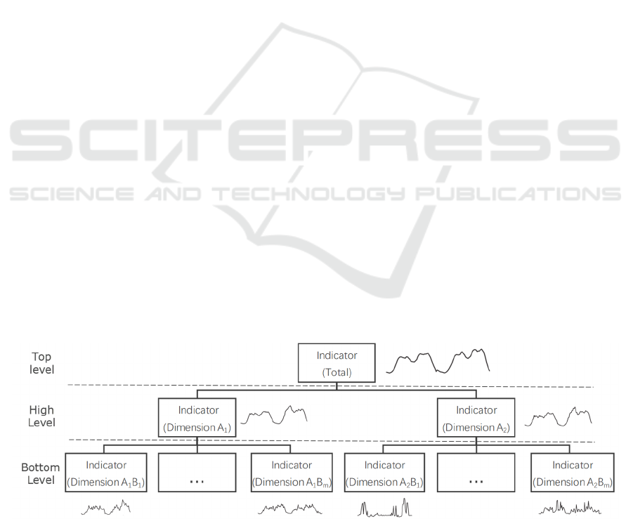
Analysing enterprise operating indicators can

facilitate the operational optimization of enterprise to

some extent. In terms of time domain, enterprise

operating indicators usually exist in the form of a

collection of time series with a hierarchical structure.

As shown in Figure 1, the total indicator can be

disaggregated in multiple dimensions. In this

hierarchy, the high-level time series is obtained by

aggregating the low-level ones which belongs to the

specific dimension.

Unlike the common single time series

prediction, hierarchical enterprise operating indicator

prediction need to satisfy the aggregation consistency

constraint between levels: the upper-level forecast is

equal to the sum of the corresponding low-level ones.

The forecasts of hierarchical time series are essential

to the elaborate management and planning for

enterprise. In this hierarchy, the decision maker likely

focus on the high-level forecasts and their root cause

analysis. In addition, multi-level drilling analysis of

anomaly enterprise operating indicator is another

important issue for enterprises management. Its main

purpose is to detect anomaly nodes in hierarchy from

top to bottom. Solving the above issues is beneficial

for decision maker to accurately and quickly find out

the operational problems.

In this paper, hierarchical prediction and root-

cause positioning algorithm are combined to form a

multi-dimensional analysis method on hierarchical

time series, which is applied in planning and

monitoring for enterprise operating indicator. The

specific contributions are summarized below:

Figure 1: The hierarchical structure of enterprise operating indicators.

716

Pang, Y., Pan, J., Li, X., Zheng, J., Sun, T. and Li, Q.

Exploring Enterprise Operating Indicator Data by Hierarchical Forecasting and Root Cause Analysis.

DOI: 10.5220/0010900500003122

In Proceedings of the 11th International Conference on Pattern Recognition Applications and Methods (ICPRAM 2022), pages 716-721

ISBN: 978-989-758-549-4; ISSN: 2184-4313

(1) In the aspect of accuracy and efficiency, a suitable

time series prediction method is adopted for anomaly

detection.

(2) Based on these prediction, the idea of root-cause

analysis method is applied in quantifying the effect of

the low-level anomaly nodes in the two-level

hierarchy. Experimental results validate the

effectiveness of root cause analysis method on

Enterprise operating indicator data. This work is

beneficial for monitoring the company's operating

indicators, and provides alert.

2 RELATED WORK

The related works mainly include hierarchical

forecasting and root cause analysis.

2.1 Hierarchical Forecasting

Classical forecasting, namely single time series

forecasting, is also called base forecasting (BASE)

(Hyndman et al., 2011). Compared to classical base

forecasts, hierarchical forecasts meet aggregation

consistency, but always at the cost of prediction

accuracy. The mainstream hierarchical time series

forecasting methods include bottom-up, top-down,

and optimal combination (Athanasopoulos et al.,

2020). In terms of computational efficiency, the top-

down predictions have the highest efficiency.

2.2 Root Cause Analysis

Key Performance Indicators (KPIs) are important

monitoring metrics for enterprise operating, which

can be divided into sequences according to multiple

dimensions. For example, page click-through rate is

an important KPI for monitoring service performance

of some internet enterprises, whose dimensions are

usually operator and accessing region. When the

overall value of KPI (root node) is abnormal, how to

trace its cause at various dimensions (child node) is

the key to maintaining good enterprise operation. To

this, some related work has been carried out.

Adtributor is proposed to locate cause by computing

its explanatory power and surprise, assuming that the

disaggregation is in one dimension (Bhagwan et al.

2014). HotSpot is proposed to determine cause when

the relationships between the indicator with

dimensional combination and its child nodes meet the

condition of ripple effect (Sun et al. 2018). Squeeze

is proposed to locate anomaly in a generic and robust

way, based on novel searching strategy and

computation of generalized potential score (Li et al.

2019).

The existing root-cause analysis method is mainly

applied in the field of advertising system, industrial

maintenance and so on. However, the research on the

enterprise operating in the field of financial payment

is scarce. Besides, a simple forecasting model based

on time series analysis is mainly adopted in the

existing methods, assuming that the forecast value is

accurate. At this situation, considering the

characteristics of real enterprise operating indicator

data, the appropriate hierarchical forecasting method

is adopted for anomaly detection, and then is

combined with adtributor to quantify the effect of

multi-dimensional indicators to identify anomalies.

3 MULTI-DIMENSIONAL

ANALYSIS ON ENTERPRISE

OPERATING INDICATOR

Enterprise operating indicator data usually have

characteristics of periodicity and seasonal pattern. In

view of these features, this paper combines the top-

down hierarchical forecasting and adtributor to form

a multi-dimensional analysis method for forecasting

and anomaly location on hierarchical time series. The

architecture of multi-dimensional analysis method is

shown in Figure 2. Firstly, the forecasts at various

level in hierarchy are obtained via modelling

historical data. Then, anomaly detection is conducted

with the forecast value at top level. Finally, locate

anomalous causes at lower level by calculating the

effect of the anomalous lower-level nodes in

hierarchy.

To clearly introduce the method, a toy example

of hierarchical enterprise operating indicator data is

shown in Table 1. The total enterprise operating

indictor time series is aggregated into series with

multiple dimensions.

Table 1: Toy example of enterprise operating indicator.

Level

Time

Top High Bottom

total Dimension

… A

0101 25 10 15 1 … 1 1 … 6

0102 27 11 16 1 … 1 2 … 7

… … … … … … … … … …

1230 48 28 19 2 … 2 4 … 2

1231 50 30 20 3 … 3 5 … 2

Exploring Enterprise Operating Indicator Data by Hierarchical Forecasting and Root Cause Analysis

717

Figure 2: Multi-dimensional analysis on enterprise operating indicator.

3.1 Hierarchical Forecasting

In time series forecasting, hierarchical forecasting

method is applied in enterprise operating indicator

data, in order to meet their intrinsic aggregation

consistency.

(1) Base forecasting

In order to ensure the accuracy and efficiency,

LightGBM (Ke et al. 2017) is adopted in time series

forecasting. The relevant experiments are shown in

section 4.3.1. LightGBM is an efficient gradient

boosting decision tree framework, which is widely

used in machine learning tasks. Its basic idea is to

combine several weak regression trees to build a

strong tree by boosting (Freund et al. 1996).

𝑦

𝑓



𝑥





(1)

where x denotes training data, n denotes the number

of decision trees, and y denotes output of the model.

Especially, in order to ensure high training efficiency,

LightGBM uses histogram algorithm and leaf-wise

strategy with depth limit to greatly reduce memory

consumption. The historical time series are regard as

the training data. Besides, the multi-order delay, the

time whether it is a weekend and that whether it is a

holiday as the additional features, are also feed into

this model.

(2) Top-down based forecast allocation

The LightGBM model are respectively adopted in

predicting total series at top level, series at middle

level and bottom level. The proportion of forecast

allocation at all these levels are then obtained

according to the above predictions (Lapide et al.

2006). Then, based on the top-down strategy, the

forecasts at middle and bottom levels are updated via

multiplying the proportion by the prediction of total

time series at future time.

3.2 Root Cause Analysis

(1) Forecast based anomaly detection

In pervious part, the 95% confidence interval of the

forecast value are also computed. When real value

falls outside the confidence interval, the series at one

timestamp is remarked as anomaly.

(2) Quantification of anomalous effect

In this part, adtributor algorithm is used to identify the

time series under various dimensions at the anomalous

timestamps. Adtributor translates multi-dimensional

root cause identification problem into multiple one-

dimensional root cause location problems, and then

collects a set of anomaly elements under different

dimensions. The multi-dimensional analysis of

enterprise operating indicator can be naturally regarded

as drilling analysis of one-dimensional root cause at

multiple stages. Therefore, adtributor is suitable for

identifying the anomalous causes.

Based on adtributor, the anomalies are detected by

computing the explanatory power value of anomalous

time series at different level in hierarchy. The relevant

formula of explanatory power is as follows:

𝐸𝑃





𝑦





𝑦



𝑦



𝑦

(2)

where i and j are the i-th dimension and the j-th of

sub-indicator. 𝑦



and 𝑦



are the predicted and the

real values of sub-indicator. y and y are the predicted

and the real value of indicator. The proportion of

fluctuations of the sub-indicator in indicator is likely

larger when the explanatory power value of sub-

indictor is larger.

In the drilling process, according to (2), the sub-

indicators’ explanatory power is obtained by using

their predicted and real values. All of the anomalous

sub-indicators can be located by comparing with the

predefined thresholds. Then, sort them in descending

order, and obtain the final results.

Hierarchical Forecasting

LightGBM based time

series forecasting

Top-down based forecast

allocation

Hierarchical

Enterprise

Operating

Indicator

Data

Hierarchical forecasting

Root Cause Analysis

Forecast based root cause

Anomaly Detection

Quantification of

abnormal effect

Anomaly Root Cause

Location

ICPRAM 2022 - 11th International Conference on Pattern Recognition Applications and Methods

718

4 EXPERIMENTS

4.1 Data

We use the enterprise operating indicator data from a

financial technology company. Based on the relevant

business scenario, the data contains a hierarchical

structure with three levels: 1 series at top level, 2

series at middle level and 74 series at bottom level.

These levels’ dimensions are headquarter, type of

bank card and administration division, respectively.

The time length of all series is from January 1st, 2019

to July 31st, 2021. The observations are respectively

daily transaction count and transaction amount,

denoted by “count” and “amount”. The given

anomalous timestamp is April 18th, 2021. The related

events take place at that time, which results in the

decline of transaction count since that time. Due to

the data privacy, both of original data and results have

been processed in this paper.

4.2 Experimental Setup

The data during January 1st, 2019 to August 31st,

2020 is used for training, and that during September

1st, 2020 to July 31st, 2021 for testing. The predicted

values with 10 days are obtained by the forecasting

method at a time. Considering data privacy issues, we

use mean average absolute error (MAPE) as the

metric, which is commonly for evaluating time series

forecasting model (Wijaya et al., 2015). It can be

calculated as follows:

MAPE



𝑦,𝑦





𝑦





𝑦



𝑦









100%

(3)

where N represents the size of test data. 𝑦



and 𝑦



are

real and forecasted values.

4.3 Experimental Results

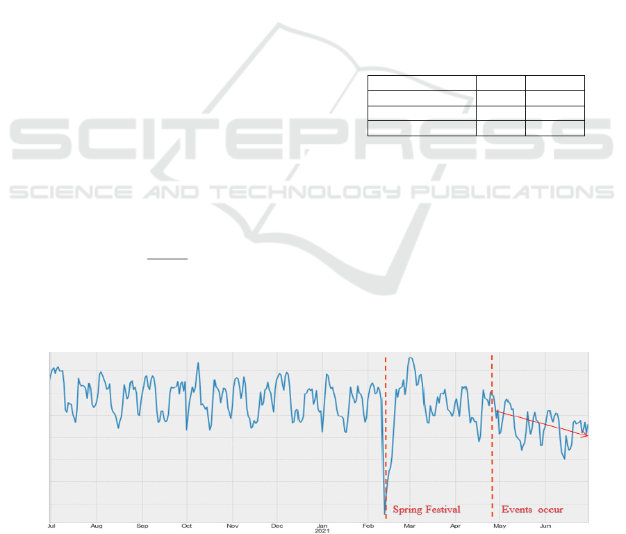
The time series analysis of data is plotted in Figure

3. Obviously, the data have the seasonal pattern, and

tend to descend since mid-April due to the related

events. The decline also occurs nearby spring festival.

4.3.1 Comparison of Forecasting Methods

As described above, indicator varies with a certain

periodicity and scale. The time series forecasting

method with the common machine learning model are

choose as baselines. The statistical model SARIMA

(Box et al. 1976) is not considered here, due to its

expensive time cost. Thus in contrast experiment,

Lasso Regression(Tibshirani et al. 2011), XGBoost

(Chen et al. 2016) and LightGBM are compared in

terms of prediction accuracy. The data without

anomalies are used, whose time period is from 2019

and 2020. The contrast results are shown in Table 2.

Table 2: The comparison of prediction accuracy obtained

by different forecasting methods.

Metho

Count Amount

Lasso Regression 4.49% 6.05%

XGBoost 3.85% 5.33%

LightGBM 3.51% 4.95%

In this table, we can see that LightGBM model

performs best on amount indicator and count

indicator. This means that LightGBM model with

historical data can obtain future trend.

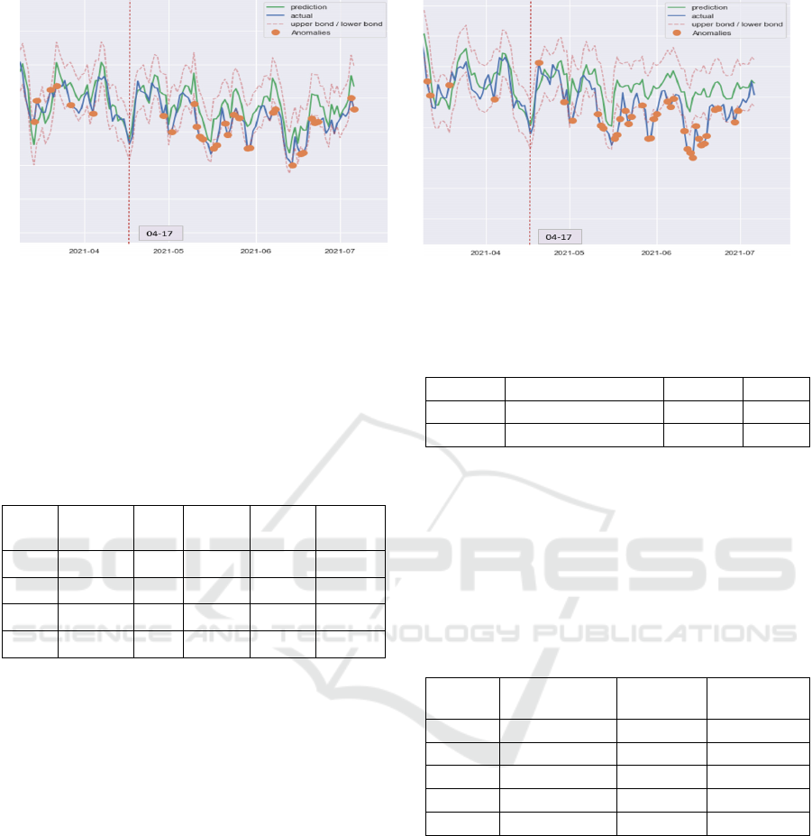
In the following experiments, count indicator is

taken as example. From the perspective of anomaly

detection, regression and LightGBM model are

compared, whose results are plotted in Figure 4. From

this figure, we can see that LightGBM can detect the

anomalies since mid-April, while regression leave out

them. That illustrates that LightGBM has better

performance in anomaly detection.

Figure 3: Time series analysis plot of enterprise operating indicator data.

Exploring Enterprise Operating Indicator Data by Hierarchical Forecasting and Root Cause Analysis

719

(

)

The detection result based on Re

ression.

(

)

The detection result based on Li

htGBM.

Figure 4: The comparison of results by Regression and LightGBM on data since mid-April.

In consideration of the lagging effect of related

events that take place in mid-April, we evaluate the

performance of the LightGBM model on data in last-

May, by computing the corresponding forecast,

confidence interval and MAPE. The results are shown

in Table 3.

Table 3: Accuracy of LightGBM for total indicator.

Time Forecast Real Lower

Bound

Upper

Bound

MAPE

0517 1.58 1.46 1.43 1.74 8.74%

0518 1.49 1.29 1.33 1.64 15.35%

0519 1.47 1.21 1.32 1.62 20.99%

0520 1.38 1.19 1.23 1.53 15.47%

From the tables, we can see that for the time on

last-May, some outliers can still be identified via

LightGBM, whose real values fall outside the

confidence interval. This is because LightGBM

model itself has the ability of noise resistance to some

degree, so that the model can still accurately capture

future pattern, even if there are noises in data. To sum

up, LightGBM is the most appropriate forecasting

model for enterprise operating indicator.

4.3.2 Root Cause Analysis

According to the description in section 3, after

detecting abnormal time of total indicator, the top-

down based forecast allocation is adopted to predicate

the sub-indicators during that time. The following

step is to apply root cause analysis algorithm to locate

anomalous indicators with the top several of

anomalous contributions. The results are shown in

Table 4 and Table 5. The effect represents the

explanatory power.

Table 4: Anomalous indicators at dimension of type of bank

card.

Number Type of Bank Card MAPE Effect

1 A

18.57% 0.97

2 A

16.59% 0.03

In Table 4, we can see that the effect of the

indicator at dimension A

is higher. That means

indicator at dimension

is probably the anomalous

cause. Next, the cause location is conducted for the

indicators at dimension of administrative division. In

Table 5, we can find out the most five possible cause

with larger effect.

Table 5: Anomalous indicators at dimension of

administrative division.

Number Administrative

Division

MAPE Effect

1 A

24.98% 0.12

2 A

20.41% 0.12

3 A

17.22% 0.08

4 A

18.96% 0.05

5 A

19.56% 0.05

Through the validation from the identified

branches respectively in

, A

and

, it is found that the results of the root cause

analysis model are in accordance with those derived

from expert experiences. These prove the

effectiveness of that the multi-dimensional analysis

method for root cause location.

In conclusion, the multi-dimensional analysis

method shows the good performance on hierarchical

forecasting and anomaly location on enterprise

operating indicator data, by effectively integrating the

suitable prediction model and quantification model

concerning the effect of sub- indicator on indicator.

ICPRAM 2022 - 11th International Conference on Pattern Recognition Applications and Methods

720

5 CONCLUSIONS

In order to strengthen the monitoring and analysis of

enterprise management and planning, this paper

introduces a multi-dimensional analysis method for

forecasting and anomaly locating hierarchical time

series, which is applied in real enterprise operating

indicators data. The suitable prediction model and

anomaly location model are adopted to automatically

identify anomalies from top to down in hierarchy.

Experimental results show that the multi-dimensional

analysis method has good performance on accuracy

of prediction and anomaly location. In future wok, we

will study on detecting of anomalous indicators with

more fine-grained indicator data.

ACKNOWLEDGEMENTS

This work was supported by the National Key

Research and Development Program of China

(2021YFC3300600), the National Natural Science

Foundation of China (92046024).

REFERENCES

Hyndman, R. J., Ahmed, R. A., Athanasopoulos, G. Shang,

H. L., 2011. Optimal combination forecasts for

hierarchical time series. Computational Statistics and

Data Analysis. 55(9), 2579-2589.

Athanasopoulos, G., Gamakumara, P., Panagiotelis, A.,

Hyndman, R. J., Affan, M., 2020. Hierarchical

forecasting. Macroeconomic Forecasting in the Era of

Big Data. 689-719.

Bhagwan, R., Kumar, R., Ramjee, R., Varghese, G.,

Mohapatra, S., Manohara, H., Shah, P., Adtributor:

Revenue debugging in advertising systems. 2014.

USENIX Symposium on Networked Systems Design

and Implementation. 43-55.

Sun, Y., Zhao, Y., Su, Y., Liu, D., Nie, X., Meng, Y.,

Cheng, S., Pei, D., Zhang, S., Qu, X., Guo, X., 2018.

Hotspot: Anomaly localization for additive kpis with

multi-dimensional attributes. IEEE Access. 6: 10909-

10923.

Li, Z., Luo, C., Zhao, Y., Sun, Y., Sui, K., Wang, X., Liu,

D., Jin, X., Wang, Q., Pei, D., 2019. Generic and robust

localization of multi-dimensional root causes. IEEE

International Symposium on Software Reliability

Engineering. 47-57.

Ke, G., Meng, Q., Finley, T., Wang, T., Chen, W., Ma, W.,

Ye, Q., Liu, T., 2017. Lightgbm: A highly efficient

gradient boosting decision tree. Advances in neural

information processing systems. 30: 3146-3154.

Freund, Y., Schapire, R. E., 1996. Experiments with a new

boosting algorithm. International Conference on

Machine Learning. 96: 148-156.

Lapide, L., Top-down & bottom-up forecasting in S&OP.

2006. The Journal of Business Forecasting. 25(2): 14-

16.

Wijaya, T. K., Vasirani, M., Humeau, S., Aberer, K., 2015.

Cluster-based aggregate forecasting for residential

electricity demand using smart meter data. IEEE

International Conference on Big Data. 879-887.

Box, G. E. P., Jenkins G. M., Time series analysis:

forecasting and control, Holden-Day, 1976.

Tibshirani, R., Regression shrinkage and selection via the

lasso: a retrospective. 2011. Journal of the Royal

Statistical Society: Series B (Statistical Methodology).

73(3): 273-282.

Chen, T., Guestrin, C., Xgboost: A scalable tree boosting

system. 2016. ACM sigkdd international conference on

knowledge discovery and data mining. 785-794.

Exploring Enterprise Operating Indicator Data by Hierarchical Forecasting and Root Cause Analysis

721